Channel depletion, LN Topology, Cycles and rational behavior of nodes

[renepickhardt]

Dear fellow Lightning developers,

at this time I believe I have rather strong evidence to explain how economic rational behavior and network topology lead to the high rate of channel depletion that we observe on the network.

Thus, I would like to share some follow up results of the mathematical theory of payment channel networks with you. Before extending the linked document I thought I collect feedback from you about two notebooks / results (notebook1 and notebook2) that I have been developing after your valuable thoughts and feedback in Tokyo.

In the afore mentioned paper I already provided a proof for the intuitive observation that cycles on the channel graph produce several liquidity states with the same wealth distribution (as a cycle usually allows for circular off-chain rebalancing, which - when neglecting routing fees - does not change the wealth distribution. Similarly it was shown with a markov model that the steady state of the LN is a spanning tree while all other channels should be depleted. I am able to come to the same conclusion but with a different approach:

Fee Potential of the Network

(The motivation why to study the fee potential will follow in the next section)

Neglecting the base fee we can define the fee potential of a node as:

\phi_v = \sum_{e\in E: v\in E}\left(\lambda(v,e)\cdot ppm(v,e)\right)

This is just the sum of a node’s outgoing liquidity in all their channels multiplied with the ppm the node can expect to earn when routing the liquidity on the channel. This is motivated by note operators who seem to maximize their fee potential.

In a similar fashion the fee potential for the entire network can be defined as:

\phi = \sum_{v\in V}\phi_v

Using integer linear programming when finding a feasible liquidity state for a given wealth distribution one could at the same time find a feasible liquidity state that maximizes \phi (or more conveniently minimize -\phi). I have done this in this notebook and made a rather interesting observation:

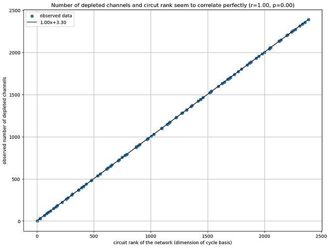
We see that the number of depleted channels in the network grows linearly with the circuit rank of the network when \phi is being maximized. Working over 10 years in statistics this is the strongest correlation on emperical data that I have ever seen. So it will be no surprise that I have a formal proof for this pattern to occur. (Disclaimer: Sidiropoulos shared a similar proof with me in a private conversation after I showed him the diagram / result).

(The circuit rank basically tells us how many more channels we have than a spanning tree or hub and spoke model.)

Why maximizing the fee potential?

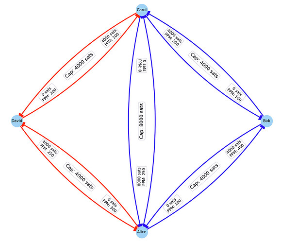
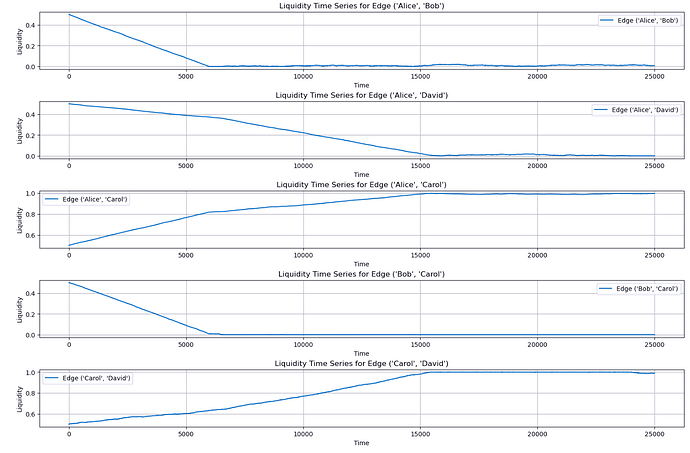
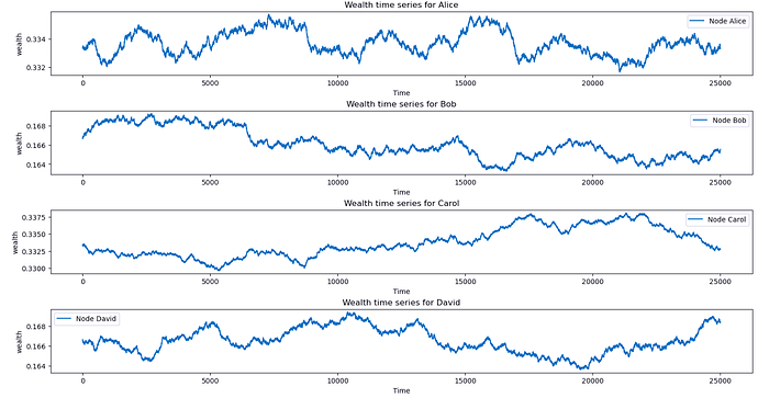
Now you could argue why should the network coordinate to maximize \phi? I was doing the same. Thus I created a small simulation in a second notebook to study if the default behavior of nodes would produce a similar state as globally solving the optimization problem.

For this I assumed the network to be initially in a random state and that nodes send each other money. For sending money the agents in the simulation will use liquid payment routs that minimize their cost. Without loss of generality I choose just the ppm as a cost function for the min cost flow computation.

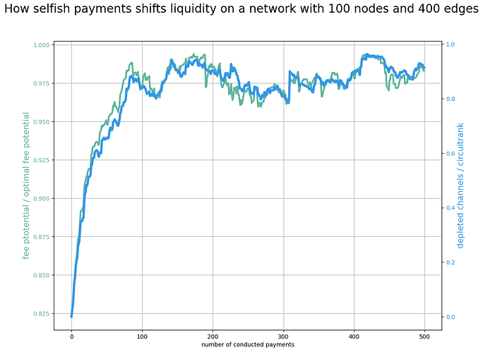
After every simulation step I computed the networks fee potential \phi and compare it with the maximized \phi potential. Similarly I looked how many channels are depleted and compared it with the circuit rank of the network.

One can see that very quickly the network reaches a state in which the network’s fee potential is very close to the maximized fee potential. Similarly almost as many channels as the circuit rank (which is the number of cycles) will be depleted.

Do we know which channels deplete?

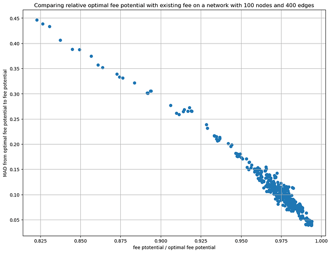
Just because \frac{\phi}{\phi_{opt}}\sim 1 does not mean that the liquidity states are actually similar. Therefor in a final step I computed after each payment also the mean absolute deviation of the current liquidity state and the one that maximizes \phi.

As you can see, only through sending payments the network converges to a liquidity state that can easily be predicted by just solving the integer linear programming problem of maximizing the fee potential with the data from gossip.

With respect to privacy: Yet again I am surprised how much information (in this case about liquidity) we can learn from gossip and the default behavior of software clients.

Limits, Conclusions & Open questions:

I am aware of a few limitations and have some open questions. There is probably more.

Limits:

• Of course the actual distribution of the liquidity depends on the assumed (but unknown) wealth distribution
• In Reality implementations use various cost functions while the simulation only used one.
• While payment dynamics are part of the model the network topology and fees are assumed to be static.
• I used uniformly distributed random payment pairs and uniform payment amounts from 0 to the max flow between the pair. (While unrealistic, I hope it does not change the emergent phenomenon but maybe only the speed with which the phenomenon emerges)

Conclusions

• Most likely much less probing will be necessary to estimate where the liquidity is located
• A spanning tree of non depleted channels remains. This is pretty much a hub and spoke topology.
• The direction of the drain of a particular channel depends on the topology and fees within the entire network (and payment flows). In particular it the ratio of ppms in both directions may be less indicative.

Open Questions:

• Is this evidence enough to conclude that drain on channels and depletion does not come from the existence of sink / and source nodes but would also emerge in a circular economy?
• Can one derive strategies for node operators to adopt fees in their liquidity management strategies?
• Are more channels than a spanning tree useful? I mean obviously they provide redundancy but also depeletion and have on chain cost.
• Similarly, how stable is the location of the spanning tree while the wealth distribution changes.
• Could the bimodel prior that is being used by many implementations be changed to one that estimates liquidity to be on one side or is it useful as the dynamic often changes the side where the liquidity will be located?
• How does the situation change if sending nodes use this knowledge to predict where liquidity is located while solving the optimization problem to send payments?
• Has anyone a good data set to test how accurate the prediction is in comparison to the actual network?

[ajtowns]

For a given initial network state, is the resulting spanning tree reproducible/predictable? Are there circumstances where the spanning tree change after being established, solely due to payments being made, without opening/closing channels (or changing fee rates)?

This seems to me like a bit like you’ve designed a network with an implicit “most expensive” spanning tree, and that the simulation simply exhausts all the cheaper paths until that’s what’s left?

Having the network spontaneously resolve itself to an acyclic spanning tree seems similar to things like amoeba maze solving or electricity finding the path of least resistance to me.

Are some nodes themselves running out of lightning funds? You could perhaps modify your simulation to address that, eg “I’m receiving $10000 a month, some by lightning, some by fiat rails; I’m likewise spending $9000 a month; if my lightning balance is $50000 or more, I’ll try to send all my payments via lightning; if it’s $25000, I’ll only try to send half my payments via lighting”.

If lightning is always your first choice when sending payments, then hitting a balance of $0 will mean as soon as you receive $50, you’ll send it right back out, so will stay depleted, which isn’t a good strategy if you want to get any value out of participating in lightning. The above might be a simple way of modelling a better one?

[renepickhardt]

@ajtowns

For a given initial network state, is the resulting spanning tree reproducible/predictable?

I am not sure I understand your question correctly. My post said we can for a fixed wealth distribution predict the location of the spanning tree by solving the integer linear program. So I guess the answer is: Yes, if we knew the wealth distribution of coins on the network.

@ajtowns

Are there circumstances where the spanning tree change after being established, solely due to payments being made, without opening/closing channels (or changing fee rates)?

That I am not too sure about and I also listed it as an open question in my OP. Thus the following is mainly a summary of observations and conjectures:

Of course the initial wealth distribution has an impact to which channels deplete. For example, if I send away all my funds, then consequently all my channels will be depleted. But as that is an extreme state I would guess with fixed topology / fees the location of the spanning tree should be somewhat stable if arbitrary wealth distributions are being picked to test for this.

Actually I tried to adopt my code to track the location of the spanning tree while the wealth distribution changes (e.g. payments are being conducted). So far my impression is that the location is less stable than I would expect. E.g. Channels which are often not depleted are still depleted in about 50% of all tested wealth distributions. (Other channels are depleted much more frequently)

Somehow this makes sense as in my original simulation the network was never in the optimal fee potential state but only close to it and a payment changed the wealth distribution.

My problem: I haven’t found a good statistical measure / visualization for that yet. I will need more time to come back to that question.

@ajtowns

This seems to me like a bit like you’ve designed a network with an implicit “most expensive” spanning tree, and that the simulation simply exhausts all the cheaper paths until that’s what’s left?

No, I don´t think that is an accurate summary / description of what I tried to present.

Just to be clear I haven’t designed a network. I just tried to find a way to explain the emergent phenomena of channel depletion that most people observe and report about.

Once I understood that the existence of different cost cycles are the reason I found it quite simple to explain:

1. Imagine the network topology was actually a spanning tree to begin with. If Alice wants to pay x sats to Bob and then Bob wants to return those x sats to Alice the network would be back in the initial state (as every wealth distribution corresponds to exactly one liquidity state in a spanning tree)
2. Now, if on the other hand the network had cycles and the fees on the edges vary it is very likely that the flow of x sats from Alice to Bob goes along a different route than the return payment. (E.g. in the example below Bob would pay Alice via Carol)
3. Thus, the payment back and forth would actually flows along a cycle and contribute to deplete that cycle.
4. In particular depletion takes place even if we don’t have source and sink nodes.

Take a look at the following extreme example:

Assume initially in the network every node has half of the capacity on their side and now nodes randomly send each other one sat.

The network will converge to the following state:

This is very interesting for several reasons:

1. All channels deplete (while all nodes keep roughly the same amount of total coins)
2. The red channels are those where the liquidity is on the cheaper end of the channel (contradicting your intuition that I have just created a “most expensive” spanning tree.
3. In fact, it is the global topology (including fees) and actual payment flows that defines which channels deplete (on which end)

For completeness I will also post the time series of how the liquidity shifts in those channels while 1 sat payments are randomly conducted between the peers:

Again it is interesting to note that it is not the cheapest 0 ppm channel that depletes first. (Makes sense at it also has twice the liquidity) but in this particular case it depletes at the same time as the other channels.

@ajtowns

Are some nodes themselves running out of lightning funds?

As just laid out, in the above example nodes have not run out of funds. I will add the zoomed in view depeicting how the wealth of each node progresses over time while the 1 sat payments deplete the channels:

Note if you zoomed the y-axis to [0,1] then you would visually just see streight horizontal lines.

Maybe I should have explicitely made the conclusion in my OP that:

• Channels deplete even if the netflow of all nodes is 0. No Source and Sink nodes are needed. Which I find quite remarkable and seems to be routed in the existance of cycles with varying costs.

@ajtowns

You could perhaps modify your simulation to address that, eg “I’m receiving $10000 a month, some by lightning, some by fiat rails; I’m likewise spending $9000 a month; if my lightning balance is $50000 or more, I’ll try to send all my payments via lightning; if it’s $25000, I’ll only try to send half my payments via lighting”.

If lightning is always your first choice when sending payments, then hitting a balance of $0 will mean as soon as you receive $50, you’ll send it right back out, so will stay depleted, which isn’t a good strategy if you want to get any value out of participating in lightning. The above might be a simple way of modelling a better one?

I am not sure about your proposed simulation. Of course I see the point that in reality people may chose between various payment rails and also onchain and ofchain payments and act acording to their liquidity requirements. But even in that world the LN graph is a somewhat closed system (with potentially less demand as some is taking place via other payment rails). In any case as laid out the phenomenon of channels to deplete seems to emerge because of various fees and the existence of cycles even if the netflow of all nodes in the network is 0.

Instead of focusing on such a mixed model wouldn’t it be more interesting to focus on how node operators should adjust their fees to help with flow control and adjust to channel depletion? Also Sending nodes could eventually adopt their route selection to use that knowledge to more quickly deliver payments.

@ajtowns

Having the network spontaneously resolve itself to an acyclic spanning tree seems similar to things like amoeba maze solving or electricity finding the path of least resistance to me.

Yes, the math that I use here to model and understand the emerging phenomena of the LN is also used to model electrical grids and other fluid networks. Intuitively it makes sense that it is also applicable in the amoeba maze solving (which I wasn’t aware of so far).

[ajtowns]

@renepickhardt

• The red channels are those where the liquidity is on the cheaper end of the channel (contradicting your intuition that I have just created a “most expensive” spanning tree.

Ah, don’t worry; I misunderstood the “spanning tree” part entirely.

In your example there are two cycles remaining: (B pays A pays C pays B), and (D pays A pays C pays D) – I think my intuition is more along the lines of those being the minimally most expensive cycles? Is there such a thing as a spanning cycle, ie a cycle that touches every node? In this case I think my intuition would be that the remaining spanning cycle CDACBAC is more expensive than any other possible spanning cycle? (Perhaps provable by noting that any payment along that cycle will create a cheaper spanning cycle, providing a cheaper path from some node X to Y, than existed previously, so the next payment from X to Y will break that cheaper spanning cycle?)

@renepickhardt

I am not sure about your proposed simulation.

Agreed: that would only be interesting if nodes were ending up depleted, rather than just channels.

@renepickhardt

Instead of focusing on such a mixed model wouldn’t it be more interesting to focus on how node operators should adjust their fees to help with flow control and adjust to channel depletion

I think you’ve already “solved” this (ok, without proof, perhaps)? The only way you avoid channel depletion is if your channel appears in the “spanning tree in which the network is balanced”, so you either need to be structurally critical, or manage your fees with far more precision than is reasonably feasible. Otherwise you’re just trying to drive straight by alternating between steering hard left and hard right… which okay, it might work, particularly if you can make the adjustments at high frequency, but sure seems pretty annoying.

To me, it makes sense that a policy of “everyone will keep using the cheapest path that works” will naturally exhaust the cheapest channels until the only ones that work are the “most expensive”, per some global metric.

To me, it seems logical that the only way to avoid that resulting in channel depletion and routing errors/retries, is to have some way of having some payments “not work” for reasons other than channel depletion, in a way that is predictable when constructing the payment route. I continue to think max_msat valves are the way to solve this.

Actually an additional thought on that topic: as a forwarding node, if you advertise a max_msat value, then you could/should use that (or a small multiple of it) as a cap on the total value of payments you’ll allow to be (recently) pending across that channel. If (in the usual case) the payment resolves “immediately” that’s no constraint at all, which is great; but if someone splits their payment into 100 max_msat HTLCs and forwards them all over your channel, you’ll immediately reject almost all of them, so there’s ~no advantage in users attempting to finesse the signal to minimise fees. (“recently” – if a payment has been unresolved for more than a few seconds, it’s probably hung, and you don’t want to continue to reject new payments because of it).

[sorukumar]

Thank you for this comprehensive work. Had an amazing last couple of days going through notebooks, linked papers and discussions

While I am in awe of the scope of the work, my comment is more around being conservative on making conclusions. While it is tempting, let’s not get carried away by sexy maths and good looking charts.

We are thoughtful on listing out the limitation of the model, but underestimating how critical they are. More so, because, we don’t have good grasp or theory on how they can ‘change’ the conclusions.

Of course some of the conclusions will continue to make sense. I’ll go on to add that number of insights tell us more about the constraints of the model rather than the lightning network. (This applies to Guidi’s otherwise excellent work as well).

To illustrate this, I’ll focus on a ‘part’ of the one of the listed limitation.

@renepickhardt

• While payment dynamics are part of the model the network topology and fees are assumed to be static.

Fee:

Fee is one of the most effective levers for node operators to manage balance of the channel.

Currently Fee potential defined as

@renepickhardt

ϕv=∑e∈E:v∈E(λ(v,e)⋅ppm(v,e))

Modeling liquidity and channel depletion with static fees is like evaluating a baseball pitcher with their throwing arm tied. it might lead us in wrong direction if we’re not careful.

A rational node operator optimizes for ‘lifetime fee value’ (LTF) of a channel. The levers of LTF: Channel Capacity, Channels own fee policy, Fee policies of adjacent channels (same node)

Potential input for the fee part of the fee potential:

1. Liquidity level and/or liquidity share of the channel

2. Peer’s fee policy for the channel

3. Fee & liquidity share of node’s other channels preceding and following in potential paths

Of course, incorporating all these factors may make the model too complicated for initial work, but at least we should have dynamic fee.

I’ll argue that no channel will ever get depleted if a we have rational/smart node runners.

• In liquidity-share aware fee models, fee rates approach infinity as the channel’s liquidity is getting towards depletion on one side. Consequently, channel unusability is triggered by prohibitive fees rather than absolute liquidity exhaustion
• Why do we have depleted channels now? It is because only few nodes are professionally run, and we don’t have good fee management algo/tools yet.

by the way, happy that fee is already in the scope of work now:

@renepickhardt

Instead of focusing on such a mixed model wouldn’t it be more interesting to focus on how node operators should adjust their fees to help with flow control and adjust to channel depletion?

Given the depth and breadth of ideas presented, I’ll tackle only open questions and conclusion with quick responses, and go deeper if there is interest.

Open Questions:

@renepickhardt

Is this evidence enough to conclude that drain on channels and depletion does not come from the existence of sink / and source nodes but would also emerge in a circular economy?

Is this evidence enough: No, not at all. Will channel depletion will emerge w/o channel management. Yes, it will.

@renepickhardt

Can one derive strategies for node operators to adopt fees in their liquidity management strategies?

Yes, an area that is as important as any other work.

@renepickhardt

Are more channels than a spanning tree useful? I mean obviously they provide redundancy but also depeletion and have on chain cost.

Pls don’t ask this. We are asking this cuz we are going too far with a simple model with number of constraints. In real world it does not make sense.

@renepickhardt

Has anyone a good data set to test how accurate the prediction is in comparison to the actual network?

Not sure what you are looking for. But, I may have some data

Conclusions

Most likely much less probing will be necessary to estimate where the liquidity is located.

Yes, may be. But other factors would also have play on it.

A spanning tree of non depleted channels remains. This is pretty much a hub and spoke topology 3.

This is very loaded question and conclusion, and may need ‘qualifications’.

The direction of the drain off a particular channel depends on the topology and fees within the entire network (and payment flows). In particular it the ratio of ppms in both directions may be less indicative.

Yes, true. However, On the ratio of PPM in both direction, it may not be indicative now, cuz most of the nodes are run as hobby projects. For professionally managed nodes when they get smarter, it will be even more indicative than it is now.

[ZmnSCPxj]

@ajtowns

(“recently” – if a payment has been unresolved for more than a few seconds, it’s probably hung, and you don’t want to continue to reject new payments because of it).

Seems gameable if the payer is willing to wait — they could release a shard below max_msat, wait, release another shard below max_msat, wait, etc. until they have 100 HTLCs through it, especially with fee_base=0 and proportional fees rounding down. Gets even worse with PTLCs since those are not correlatable.