[Research] Vardiff belongs at the frontier
A note on where this came from. This is the companion to “A clockless vardiff strands a slowing miner.” That post asked whether a single controller is decline-safe; this one asks a prior question — where in a mining topology does difficulty control belong at all, once the miners sit behind proxies, translators, and job-declaration clients rather than dialing the pool directly. It was worked out through an extended back-and-forth with an AI (Claude), with ideas going both ways; the direction, the judgment calls, and the verification are mine. The claims here rest on two things, and I mark which throughout: direct review of the deployed Stratum V2 source (the reference pool, translator, and JD-client), and the counting/observability argument from the earlier post. Where a claim is neither — where it is a structural conjecture I have not measured — I say so. One deployed third-party pool (Blitzpool) is cited from its public source as an independent witness.
The question
Picture the simplest case: one miner, one pool, difficulty set on the one channel between them. The earlier post lived here — one controller, one decision. But almost no real deployment is this simple. Miners sit behind a translator that speaks SV1 downward and SV2 upward; behind a job-declaration client that brings its own block templates; behind a proxy that collapses many miner connections into one upstream connection. Difficulty is no longer one decision on one link. So the question this post answers is: when the path from miner to pool passes through intermediate nodes, where does difficulty control actually live — and where should it?
A word on what kind of claim this is, because it shapes everything below. This is a method — characterize a controller by the constraints its domain imposes — applied a second time. Paper one turned it on a single vardiff controller: a share stream carries no information during silence, so a decline-safe controller must ease on the clock, not on shares. This post turns the same method on the topology — once the path from miner to pool has structure, what does that structure force about where control can live? The reasoning runs from the observability of the tree, not from any one implementation. Stratum V2 is the instance I test it against: the deployment I can hold the derivation up to and check against source. And the part I didn’t expect is how closely the reference stack already conforms to what the derivation says it should. But that alignment is a finding, not the goal — the argument would hold for any topology with this structure, and SV2 is simply where I could confront it with real code.
The way in is to start with the one-server case and insert a second server, one step at a time, and watch what the change does to the estimation problem underneath. The structure that has to exist falls out of that — including where difficulty control is forced to live, and why.
1. One server: one loop per miner
When a miner dials a pool directly, difficulty control is doing exactly one live job: track this miner’s rate and set its difficulty so it submits at a good cadence, neither starved nor flooded. That’s the per-miner health loop — the decline-safety controller of the earlier post — and it runs continuously because the miner’s rate moves.
When the pool sees each miner directly, that’s the whole of it: one tracking loop per miner. The total — “how much hashrate is arriving” — isn’t a separate tracked quantity: the pool already tracks every component, and the total is just their sum.
2. Insert a second server, and the estimation problem changes
Now put a proxy between the miners and the pool. A proxy collapses many miner connections into one upstream channel — fewer connections for the pool to terminate, which is often the point. A given proxy aggregates its own miners. But whatever the reason, the moment a proxy multiplexes its miners onto one channel, the estimation problem on that channel changes. Ask the concrete question — what can each node now measure?
-
The proxy still sees each of its miners’ own share streams, clean and separate. Per-miner rate is estimable there.
-
The pool no longer does, for that channel. Each miner’s shares still cross the upstream link — they aren’t dropped, merged, or re-minted — but they arrive multiplexed onto one channel, and the pool’s difficulty controller tracks that channel as a single pooled stream. So what it can estimate well is the channel’s aggregate rate (more shares, tighter estimate); any single miner’s contribution is 1/N of that pool, under a noise floor that (by the counting law from the earlier post) fell only by \sqrt{N}. One of that proxy’s miners slowing down is invisible in the pooled count. (Verified from source: in aggregated mode the proxy forwards every valid share onto one upstream channel with a single share counter — the individual shares survive, but the controller counts them together.)
So adding the proxy did two things at once, for its channel. It put the per-miner signal out of the controller’s reach: the clean, separable per-miner streams the difficulty loop needs now exist only at the proxy. (The share events do reach the pool — and stay attributable to a miner for accounting — but the difficulty controller counts them per-channel, so for control the per-miner rate is gone above the proxy.) And it created a new quantity that didn’t exist before — the aggregate rate of that proxy’s subset, a distinct thing from any single miner’s rate, visible only at the pool. When the pool saw those miners directly, their “total” was just the sum of components it already tracked; behind the proxy it’s a separate quantity, and it moves on its own — up and down as miners join, leave, and change their own hashrate. And a topology can hold several such proxies alongside direct miners, so the pool ends up terminating a mix: some aggregate channels, some per-miner.
3. The split forces a second loop into existence
Follow the predicament the second server created. We started with one per-miner loop and nothing else to track. Now:
The aggregate rate has to be tracked. That new quantity — the summed rate of the proxy’s subset, crossing the upstream link — drifts as those miners come and go and change their own rates. So the channel’s difficulty has to follow it: a target set once is already wrong the moment the subset shifts — too easy once the aggregate grows and floods the channel, too hard once it shrinks and starves it. A tracking job has appeared that wasn’t there before — when the pool saw those miners directly it tracked each as a component, and had no separate total to chase.
But the loop we already have can’t stretch to cover it — and this is the crux, because it’s can’t, not shouldn’t. Control follows signal: a controller can only track what its vantage point can see. The two moving quantities now live at two vantage points, neither of which can see the other’s:
-
The per-miner rates are visible only at the proxy (above it, they’re pooled onto one channel and no longer separable). So the existing per-miner loop is forced down to the proxy — the pool cannot run it, having nothing to estimate a single miner’s rate from.
-
The aggregate rate is visible only at the pool (the proxy sees individual streams, not the total the pool receives on one channel). So the new tracking job can only run at the pool.
One controller cannot track two moving quantities it cannot simultaneously see. The per-miner loop, forced to the proxy, is blind to the aggregate; a controller at the pool, seeing only the aggregate, is blind to the miners. So the new tracking job cannot be absorbed by the existing loop — it must become a second loop, born at the pool, forced into existence by a moving quantity appearing where the first loop can’t reach.
One caution, because this new loop is easy to mistake for something the pool already had. A pool has always set an accept-threshold — a minimum difficulty it will credit at all, set once for its own bandwidth and accounting reasons. That is not a loop; it’s a static floor that chases nothing. The aggregate-tracking loop is a different animal: it actively follows a moving quantity. So don’t conflate them — the second loop is a new tracking controller, born at the pool from the split; the accept-threshold is a standing static bound that was always there.
4. The line that split them has a name: the frontier
Step back from the two loops and look at what created them. The per-miner loop was forced to the proxy because that’s the last place the per-miner signal survives. One hop further up, it’s gone. So there is a line in the topology — the boundary past which the per-miner signal no longer exists — and the per-miner controller must sit at or below it. Call that line the frontier. The frontier is a line; a node is the frontier when that line runs through it. An aggregating node reads its miners’ separable streams and only then pools them, so the line falls inside it: the controller sits on that node while reading the still-separable view just below the line — which is why “on the frontier” (the node) and “below it” (the line) name the same seat.
The frontier isn’t a concept imposed on the problem; it’s the name for the line the split exposed. Placement, then, is not free: control cannot sit above the frontier — nothing past it can estimate a single miner’s rate. How tight that bound is depends on the node. Where a node degrades the signal, there is nowhere higher to run, so the seat lands on the frontier itself. Where the path is pure pass-through, the frontier rides up to the pool, and which node below it actually runs the loop is a control decision the next sections take up.
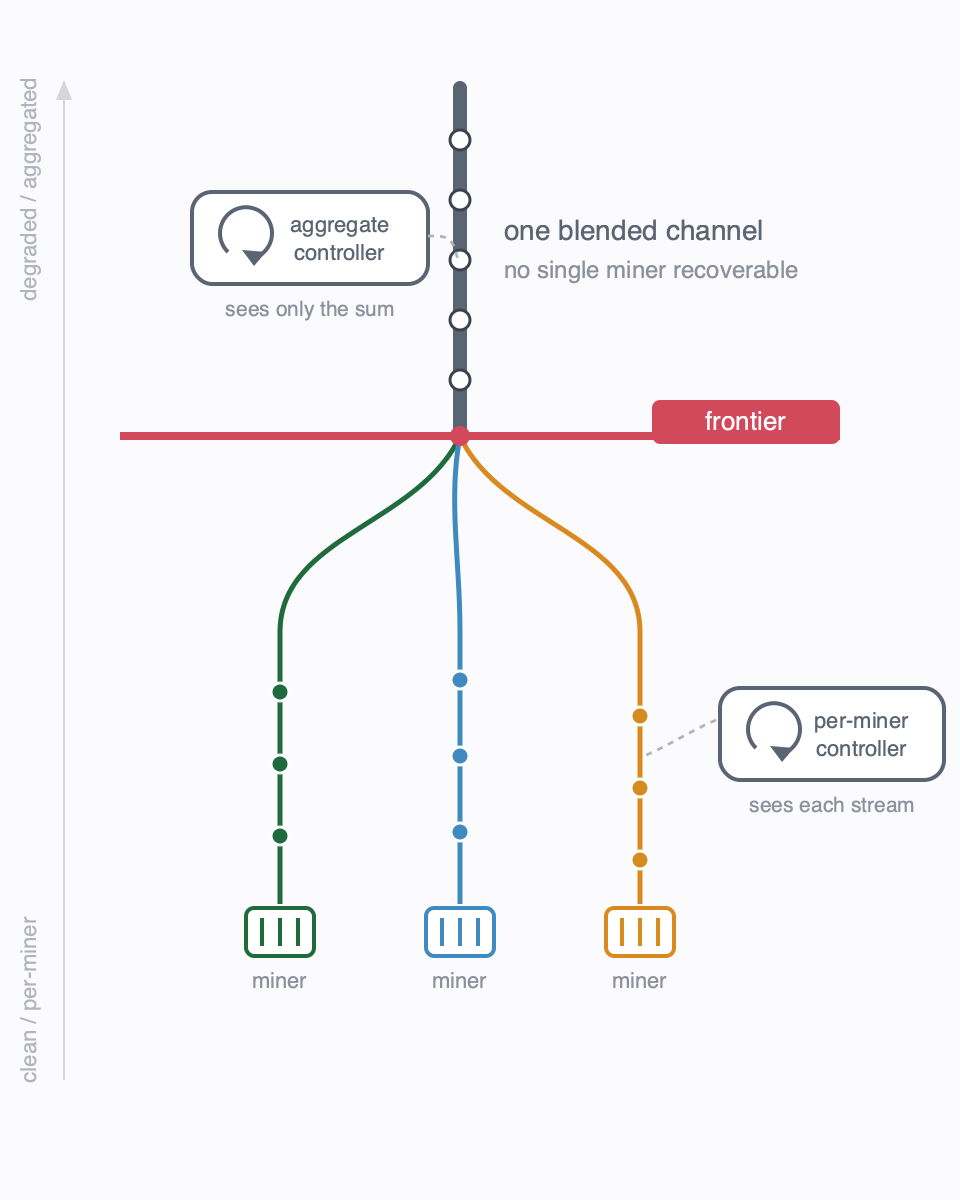
Below the frontier, each miner’s share stream is distinct and individually estimable; above it, the streams are multiplexed onto one channel and no single miner’s rate is recoverable by the controller. The per-miner controller must sit below the frontier — the only place its signal is separable. (Shown for aggregation; filtering and censoring degrade the signal by different means but define the frontier the same way.)
We derived the frontier from an aggregation split — the proxy multiplexed the streams onto one channel. But the frontier isn’t really about aggregation. What mattered was only that the per-miner signal stopped being separable to the controller above the boundary — and multiplexing is just one way to make it inseparable. A node can degrade the per-miner signal by at least three genuinely distinct mechanisms:
-
Aggregation — multiplex many miners onto one channel (the case we just walked). No share is dropped; the controller above simply counts the pooled stream, so a single miner is 1/N of the count.
-
Filtering — forward only some shares (e.g. only those meeting a target) and drop the rest, so the node above sees a thinned stream, not the full distribution.
-
Censoring — know that share-attempts happened but decline to report them, so the upstream sees a censored stream: attempts occurred that it will never learn about.
These are not the same operation under three names — they differ in what happens to a share. Aggregation keeps every share but pools the count; filtering drops the shares below a threshold; censoring withholds known attempts. What they share is only the consequence: each changes the character of the estimation problem above it, so an estimator tuned for the clean per-miner stream is the wrong tool for any of them. That common consequence is the frontier: in general it is the last pass-through node before the first signal-degrading one — where a pass-through node preserves the separable per-miner signal and a degrading node (by pooling, dropping, or withholding) does not.
Whether a given node is pass-through or degrading can be a configuration choice. The SV2 translator is the clean example: it carries an `aggregate_channels` flag, and with it off (verified from source: “if false, each miner gets its own channel”) the translator relays each miner as its own upstream channel — the per-miner signal survives it, so it’s pass-through and the frontier sits above it. Turn the flag on and it multiplexes its miners onto one channel — now the controller above sees a pooled count, so it degrades the signal and is the frontier. Same node, and which side of the line it falls on is a setting. (Note this is a separate axis from whether the translator runs its own difficulty loop — that’s a control decision, which the next sections take up; here we’re only asking what the node does to the signal.)
Aggregation was the on-ramp; the real principle is control follows signal, and the frontier is where the signal stops being separable. (A deployed pool hit exactly this — via filtering, not aggregation.)
5. The default is a cascade, not a single seat
The derivation shows both loops must exist; the deployed source shows which one a deployment can turn off. (Verified from source.) The reference SV2 pool runs its variable-difficulty loop on every channel it terminates, unconditionally — it makes no distinction between a channel carrying one miner and one carrying a proxy’s aggregated subset. So on any aggregated topology the pool’s loop on the aggregate is always live: not optional, not a configuration choice, but the default.
What is a choice is the inner loop. The translator’s per-miner difficulty control is a toggle (its enable_vardiff setting, on by default). (Verified from source.) So the two loops §3 derived are, in the deployed stack:
-
Two live loops (the default): the proxy runs per-miner difficulty at the frontier, and the pool runs difficulty on the aggregate above it. A cascade.
-
One live loop (the special case): disable the inner loop, and only the pool’s always-on outer loop remains.
The earlier post’s “one controller, one decision” world is the special case — the configuration you reach by turning the frontier controller off.
The per-miner protection — the entire subject of the earlier post — lives in the loop a deployment can switch off. Switching it off doesn’t leave the miner unprotected-but-fine; it hands per-miner health to the pool’s outer loop, which structurally cannot see a per-miner decline: that decline is 1/N of the aggregate, buried under a floor that fell only by \sqrt{N} (§2). To make that concrete — take a proxy aggregating a thousand miners. One miner is 0.1% of the aggregate, while the aggregate rate itself carries about 1/\sqrt{1000} \approx 3\% Poisson counting noise — the same counting law as §2, just at N=1000. So a single miner’s entire contribution sits roughly 30× below the noise the pool’s estimator already lives with: not merely hard to see, but categorically beneath the resolution — like trying to hear one conversation stop by listening to the volume of a stadium. So the protection is optional, and its absence is not neutral — it’s a handoff to a controller that is provably blind to the thing being protected.
6. The telescope: extending one proxy to many
Chain the proxies — miners → proxy A → proxy B → \dots → pool — and each node faces the same pass-through-or-degrade choice, now with a consequence for the ones above it. The frontier is wherever aggregation begins: below it, separable per-miner signal; above it, only the pooled count. So the frontier isn’t fixed by the topology’s shape — it’s set by which node aggregates first, and it pushes up as long as nodes keep preserving. A chain of pure pass-through translators leaves the frontier all the way up at the pool; the first one that aggregates claims it, and above that point no node can run a per-miner loop — the per-miner signal is gone, so any controller there acts on an aggregate. (A node above an aggregator can perfectly well be pass-through; it just forwards the already-pooled channel. What no node above can do is rebuild the per-miner signal the aggregator destroyed.)
And once aggregation stacks, the controllers form a telescope: each layer estimates the sum of everything below it. Proxy A estimates one miner; proxy B estimates A’s whole block as a single quantity; the node above B estimates B’s block; and so on up to the pool. Each layer treats the layer below’s aggregate as one input — the same operation repeated, the unit of aggregation growing at each hop.
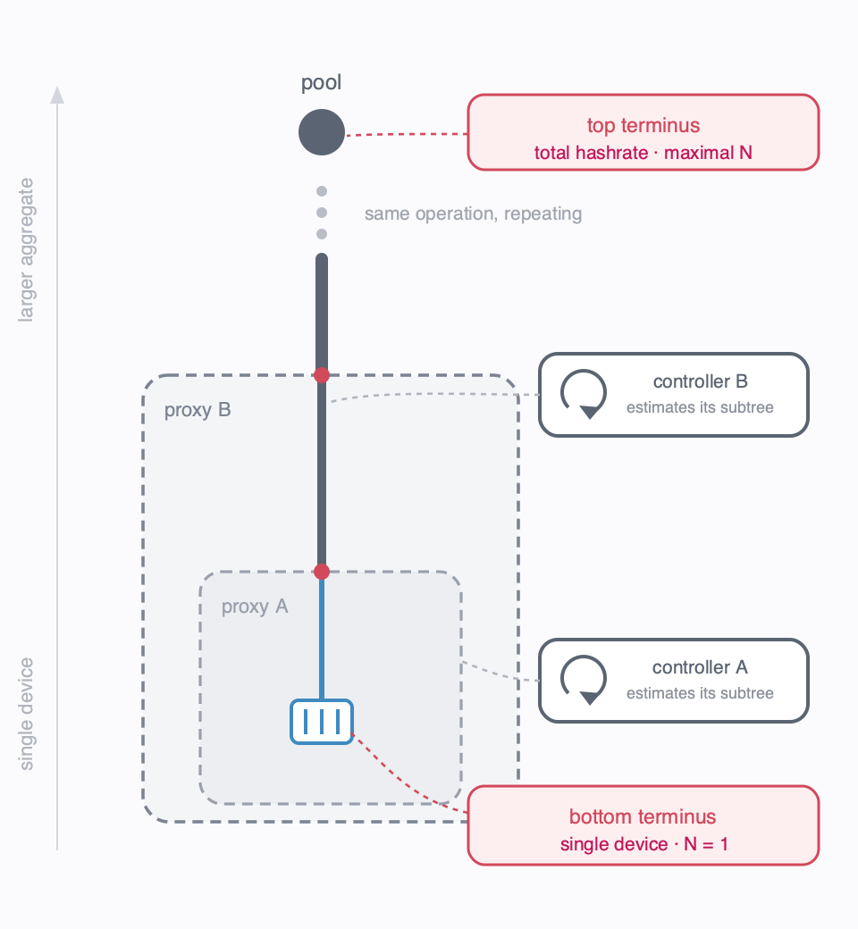
The telescope: each level estimates the sum of its own subtree, and the same operation repeats up the chain — proxy A nested inside proxy B, and so on. It ends naturally at both termini: the single device at the bottom (per-miner health, N=1) and the pool’s grand total at the top (total hashrate, maximal N).
The telescope terminates naturally at both ends, and those two ends are the per-miner loop and the aggregate loop — the original loop and the one the split forced into being:
-
The bottom is the single device. There’s nothing below one miner to aggregate — its own stream is the finest clean signal there is. This is the per-miner health loop, the one that existed from the start (§1).
-
The top is the pool’s grand total. You can’t aggregate above everything. This is the aggregate-tracking loop taken to its limit — the whole-farm total, the moving quantity a second server first made distinct (§3), best answered at the pool with all the shares.
Each node is the best available estimator of its own subtree: it sees exactly the miners beneath it, summed into one stream. That gives it more shares to work from than any single miner has alone — a tighter estimate of the subtree’s total — and it sees that subtree before it is blended with others, which no node above it can. The proxy estimates its subset best; the pool estimates the total best. So the topology is a map of which node can best answer which hashrate question: to read the hashrate of any group of miners, the right place to ask is the node whose subtree is exactly that group. Per-miner health and pool total are just the two ends of that map — the smallest subtree and the largest — and wherever the tree runs deeper, the same holds at every level in between.
Read the other way, the same map localizes trouble. An anomaly in the pool’s total is a statement about the whole tree; to place it, descend — at each level follow the child subtree whose estimate moved, drop the ones that didn’t, and narrow the disturbance to the smallest subtree that still shows it. But only that far: below an aggregating node the per-miner streams are pooled, so a fault localizes to the aggregate and no finer. The frontier bounds diagnosis exactly as it bounds control — the same separability decides where a controller can sit and how sharply a fault can be placed.
(This structure is a conclusion from the verified pieces above — the observability argument, the pool-runs-on-every-channel fact, the counting law. What I have not verified is that real deployments build deep telescopes; the prevailing assumption is that flatter topologies are preferable, and I have no source on how deep production farms stack. So the telescope is presented as the structure the protocol admits, not a claim about what farms commonly build.)
7. Blitzpool: the principle deployed — via filtering, not aggregation
The frontier isn’t only a tidy idea — a production pool already runs on it, and via a different degrading boundary than the aggregation we derived it from. (Cited from Blitzpool’s public source.) Blitzpool ships two different difficulty algorithms at two points in its topology:
-
On its ordinary path — where it sees each miner’s full share stream — a sliding-window estimator over the share distribution.
-
On its job-declaration path — a count-based estimator that watches how many shares arrive per interval rather than their full distribution.
And its own code states why, in an operator’s words: the sliding-window algorithm doesn’t work for a job-declaration client because the pool no longer sees the full share distribution — the JD-client filters shares against its own target and forwards only those that meet it, so the pool sees a thinned stream and instead counts the shares it does see.
That is the frontier principle, deployed — but reached through filtering, not aggregation. (Verified against the SV2 JD-client’s own source, not only Blitzpool’s description: sub-target shares are rejected, not passed up — the ordinary per-channel target check, one hop up, which makes it a clean instance of a signal-degrading boundary.)
So Blitzpool matches its estimator to the surviving signal at a degrading boundary — the frontier, in the wild. And the two paths reach that boundary by mechanically different means: the telescope’s aggregation keeps every share but pools the count, while Blitzpool’s JD-client path drops the shares below its target. Those are not the same operation — one multiplexes, the other filters — yet they land a controller in the same predicament: the clean per-miner stream no longer reaches it. That two unrelated mechanisms produce the same frontier is exactly why the frontier is the right abstraction: it was never about aggregation specifically, but about separability lost, however a node happens to lose it.
I should be plain about what I’m claiming and what I’m not. I’m reading Blitzpool’s design through the lens of my own framework, and inferring its intent from its source logic and code comments — the author has not told me his reasoning. On that reading the match is as clean as I could hope for: two controllers, split at exactly the boundary where the visible signal changes character, with the code comment giving the frontier’s own reason (“the pool no longer sees the full share distribution”). But that’s my inference about someone else’s system, not his stated intent, and I’d welcome his own account of how well — or how poorly — his design actually maps to this theory.
What I’m not doing here is the harder question underneath: what the right controller is on each side of the frontier — how a frontier (per-miner) vardiff should ideally differ from an aggregating one, and how two such loops behave when they run stacked in the same path. Blitzpool answers the placement question by putting different algorithms at different positions; it doesn’t tell us those are the best algorithms for each position, and I’m not claiming they are. The design of the two controllers, and how they interact when stacked, is where I suspect the interesting behavior hides — and it’s the follow-up, not this one.
8. A mismatch worth naming
The counting argument says each telescope position has a different statistical character — a clean per-miner stream and a blended N-miner sum want different estimators. Blitzpool acts on this, running different algorithms at different positions. The reference SV2 pool does not: it runs the same difficulty algorithm on every channel it terminates. (Verified from source.)
So the same estimator is applied to a per-miner channel and to a thousand-miner aggregate alike, and by the counting argument it cannot be right for both — running the per-miner estimator on the aggregate leaves precision (\sqrt{N}) on the table. Whether that costs anything in practice, I have not measured; it may be an acceptable simplicity choice or a latent inefficiency. And whether any such imprecision even reaches payouts — and if it does, whether it bites differently under PPS than under PPLNS, which place the variance the pool absorbs in different hands — isn’t answerable from what’s deployed: the reference stack stops at difficulty and share validation, with no reward-accounting layer to measure a payout effect against. So it’s a well-posed question the follow-up would need an accounting module to answer. (Conjecture on the cost and on any payout-scheme dependence; the same-estimator-everywhere fact is verified.) I name it because it’s the seam where a topology-aware difficulty design would differ from the current one — and because Blitzpool shows a deployed pool already differing there.
9. A configuration trap
The frontier is also something an operator can get wrong. The translator has two knobs that between them decide its relationship to the frontier: whether it aggregates (aggregate_channels) and whether it runs a per-miner loop (enable_vardiff). Two of the four combinations place the per-miner loop on the right side of the boundary the node creates; two fight it.
- Both on, or both off, are coherent. Aggregate-and-run-a-loop: the translator is the frontier and runs the per-miner loop there. Preserve-and-run-nothing: it isn’t the frontier, so it correctly leaves the per-miner loop to a node above it. (Coherent means the loop is placed correctly relative to the frontier — not that miners are necessarily protected. If no node runs the inner loop, you are back in the switched-off-protection case, however coherent each node is on its own.)
The two mismatched settings are the ones to watch, and they fail at different levels.
-
Aggregate on, vardiff off is a placement failure I can state firmly, because it’s the per-miner-blindness result reached by a config: the translator degrades the signal — it becomes the frontier — but runs no per-miner loop, so the loop the frontier ought to hold isn’t run here, and it cannot be recovered above, because the signal it needs is already summed away. Per-miner protection is gone. That’s not a new claim; it’s the switched-off-protection consequence, arrived at by a settings choice rather than a code path.
-
Aggregate off, vardiff on is murkier, and I flag it rather than judge it. The translator preserves the per-miner signal and runs a per-miner loop — but the signal keeps flowing up to wherever the frontier actually is, so a per-miner loop may end up running at more than one node on the same miners. Whether two such loops merely duplicate work or actively fight is a dynamics question — the same loop-interaction the follow-up takes up — so it’s a flag, not a verdict.
And beyond which combinations are coherent, there is likely a further layer I’m not addressing: relative timing constraints between stacked loops. That too is the follow-up’s territory, and I have no verified recommendation to offer yet.
10. What this is, and what comes next
The claim is narrow and, I think, solid: difficulty control belongs at the frontier — the last node before the per-miner signal is degraded — and in a real topology that means a cascade of controllers, one per boundary, telescoping from the single device up to the pool total. The frontier emerges from a concrete fact (insert a node, the estimation problem splits), not from an abstraction; placement is bounded by the topology, not an arbitrary choice — control can never sit above the frontier, and at a degrading boundary the seat lands on it; and the degrading boundary that defines it can be aggregation, filtering, or censoring. The per-miner protection lives in the frontier loop, which is the optional one, whose absence hands miner health to a provably-blind aggregate loop. And a deployed pool (Blitzpool) already matches estimators to boundary position, while the reference implementation does not.
The through-line is the one the intro set out: characterize the vardiff control problem by the constraints its domain imposes, and let the structure fall out. The single controller was paper one; the topology is this one. The SV2 reference stack turns out to sit right where the derivation says it should — the pool’s loop live on every channel it terminates, per-miner control seated at or below the frontier. I’d expected to have to argue for that placement; the deployed code bears it out. But that stays a finding about one instance, not the claim itself: the claim is about the structure, and SV2 is just where I could check it.
Three threads I’m deliberately leaving for follow-up work rather than claiming here:
-
What the stacked loops do when they run together. This paper places the loops; it doesn’t study how they behave once both are live in the same path — and I suspect that’s where the interesting behavior is. Two angles on the one question: the control angle (what the right per-miner vardiff and the right aggregate vardiff each are, and how the two interact), and the timing angle that makes the interaction concrete — multiple difficulty loops all on the same fixed cycle, with a variable delay between a downstream’s request and the upstream’s grant, which is a nested-control-loop situation with a known destabilizing shape. I can see the precondition in the deployed code — every layer runs the same fixed cycle, so there’s no timescale separation — but I have not observed the instability, and it isn’t named anywhere in the reference project. The interaction and its timing are the same problem seen from two sides; characterizing it is the follow-up, not a claim I’ll make on structure alone.
-
Censored-observation estimation. Blitzpool’s filtering boundary is, as an estimation problem, a censored one — a different operation from aggregation (§4), but kin to it in what it does to the estimator — and a proper treatment of estimating a rate from a censored share stream connects to the entrenchment follow-up. Blitzpool’s count-based estimator is a deployed instance of exactly that, which I note here and take up there.
-
The accounting cost of the mismatch. If the estimator mismatch does leave real precision on the table, the next question is whether that imprecision reaches payouts — and whether it does so differently under PPS than under PPLNS, which place the variance the pool absorbs in different hands. This one is genuinely out of reach here, not just unfinished: measuring a payout effect requires a share-accounting module, and neither this setup nor the SV2 reference stack has one — the reference implementation stops at difficulty and share validation, upstream of any reward accounting. So the question is well-posed but not answerable from what exists today; it needs an accounting layer to test against, and it’s the natural next question for whoever has one (the miners carrying the variance most of all).
The frontier is where the signal degrades; that much is structure, and it’s verified. What happens when the loops that live along it start interacting is dynamics, and that’s the next post.
Notes on sources
The control-theory and observability framing carries over from “A clockless vardiff strands a slowing miner.” The claims marked verified from source were read against the deployed Stratum V2 reference implementation (pool, translator, JD-client) and, for the Blitzpool material, against Blitzpool’s public source. The counting law (1/\sqrt{N} relative uncertainty on a Poisson share stream) is the same standard result the earlier post used. Claims marked conjecture are structural inferences I have not measured, and are flagged as such rather than left to look verified.