Cluster mempool definitions & theory

[sipa]

Cluster mempool theory

Transaction graphs and clusters

Definition. A transaction graph, or in cluster mempool context, just graph, is a directed acyclic graph (DAG), with n vertices (also called transactions), where each vertex is labelled with a fee (an integer) and a size (a strictly positive integer). If an edge from node c to node p exists, p is called a parent or dependency of c, and c a child of p. In other words, transaction graphs are dependency graph whose vertices point to their dependencies.

Definition. Given a graph G and a transaction x in it, the ancestor set \operatorname{anc}_G(x) of x is the set of all transactions which can be reached from x (this always includes x itself). For sets S, we define \operatorname{anc}_G(S) = \cup_{x \in S} \operatorname{anc}_G(x), the union of the ancestor sets of all the transactions in the set.

Definition. Given a graph G and a transaction x in it, the descendant set \operatorname{desc}_G(x) of x is the set of all transactions from which x can be reached. For sets S, we define \operatorname{desc}_G(S) = \cup_{x \in S} \operatorname{desc}_G(x), the union of the descendant sets of all the transactions in the set.

Definition. A cluster is a connected component of a graph ignoring direction. In other words, for any two transactions in a cluster it is possible to go from one to the other by making a sequence of steps, each traveling along an edge in either forward or backward direction. The clusters of a graph form a partition of its vertices, and the cluster of a transaction is the connected component which that transaction is part of. It can be found as the transitive closure of the “is parent or child of” relation on the singleton of the given transaction.

Consider the transaction graph below (fees and sizes are omitted):

graph BT
   t5["t<sub>5</sub>"] --> t2["t<sub>2</sub>"];
   t6["t<sub>6</sub>"] --> t2;
   t6 --> t3["t<sub>3</sub>"] --> t1["t<sub>1</sub>"];
   t7["t<sub>7</sub>"] --> t4["t<sub>4</sub>"];

In this example there are two clusters: \{t_1, t_2, t_3, t_5, t_6\} and \{t_4, t_7\}.

Definition. Given a subset S of nodes of a graph, define the following functions:

• \operatorname{fee}(S) = \sum_{x \in S} \operatorname{fee}_x: the sum of fees of transactions in S.
• \operatorname{size}(S) = \sum_{x \in S} \operatorname{size}_x: the sum of sizes of transactions in S.
• \operatorname{feerate}(S) = \operatorname{fee}(S) / \operatorname{size}(S): the sum of the fees divided by the sum of the sizes of transactions in S. Only defined for non-empty sets S.

Linearizations and chunks

Definition. A topological subset S of a graph G is a subset of its transactions that includes all ancestors of all its elements. In other words, S is topological subset of G iff \operatorname{anc}_G(S) = S.

Definition. A linearization L for a given graph G is a permutation of its transactions in which parents appear before children. In other words, L = (t_1, t_2, \ldots, t_n) is a linearization of G if \{t_1, t_2, \ldots, t_k\} is a topological subset of G for all k = 1 \ldots n. A linearization is thus a topological sort of the graph vertices.

In the example above:

• (t_1, t_2, t_3, t_4, t_5, t_6, t_7) is a valid linearization.
• (t_2, t_5, t_1, t_3, t_6, t_4, t_7) is a valid linearization.
• (t_1, t_3, t_6, t_2, t_5, t_4, t_7) is not (t_6 is included before its parent t_2).

Definition. Given a linearization L for a graph G, and a subset S of G, the sublinearization L[S] is the linearization of S which keeps the same internal ordering as those transactions have in L.

Definition. A chunking C = (c_1, c_2, \ldots, c_n) for a given graph G is a sequence of sets of transactions (called chunks) of G such that:

• The chunks c_i form a partition of G (no overlap, and their union contains all elements).
• Every prefix of chunks is topological (\cup_{i=1}^{k} c_i for k=1 \ldots n are topological subsets of G). Thus, a transaction’s parent can appear in the same chunk as the transaction itself or in an earlier chunk, but not in a later chunk.
• The feerates of the sets are monotonically decreasing.

Note that in practice, we will only work with chunkings of individual clusters, rather than possibly-disconnected graphs. The reasoning for that will come later, so for now, we define chunkings for graphs in general.

Definition. The function \operatorname{chunks}(L) for a linearization L = (t_1, t_2, \ldots, t_n) of a graph G returns the corresponding chunking of that linearization, defined as:

• If L (and thus G) is empty, \operatorname{chunks}(L) = ().
• Otherwise:
  • Let f_j = \operatorname{feerate}(\{t_1, t_2, \ldots, t_j) for j = 1 \ldots n.
  • Let k be the smallest integer \geq 1 such that no f_j > f_k exists.
  • Let c = \{t_1, t_2, \ldots, t_k\}.
  • \operatorname{chunks}(L) = (c) + \operatorname{chunks}(L[\{t_{k+1}, \ldots n\}]).

In other words, \operatorname{chunks} constructs the chunking of a linearization consisting of successively best remaining prefixes of that linearization.

Theorem. The corresponding chunking \operatorname{chunks}(L) is a valid chunking for G.

Proof. All criteria for a valid chunking are fulfilled:

• All transactions that occurred in L (which are all transactions in G) will appear in \operatorname{chunks}(L) once.
• Every prefix of chunks is topological, because each corresponds to a prefix of L (which are topological for any valid linearization).
• The feerates are monotonically decreasing. If that wasn’t the case, the chosen k would violate the “no f_j > f_k” rule.

Theorem. The feerate of a prefix of a linearization never exceeds its first chunk feerate. If it did, the first chunk would clearly not be the highest-feerate prefix of the linearization.

Theorem. The feerate of a suffix of a linearization is never less than its last chunk feerate. This is true within the last chunk, because if there was a suffix of the last chunk with lower feerate than that chunk, that suffix could be split off, and the feerate of the part before it would go up. It is also true across multiple chunks, because if a suffix can’t have a lower feerate than the last chunk, then extended the suffix to a chunk before it (whose maximum suffix feerate is even higher) cannot change that property.

Definition. We also define a corresponding linearization of a chunking as a linearization consisting of a concatenation of the chunks, in order, and within each chunk ordered topologically. This correspondence is not unique (because there can be multiple topological sorts of the chunk elements), but all corresponding linearizations of a chunking have the original chunking as corresponding chunking (or a strictly better one) Due to the simplicity of converting between chunking and linearization, we can often treat them as the same.

Definition. Given a chunking C = (c_1, c_2, \ldots, c_n), its feerate diagram \operatorname{diag}_C is a real function with domain [0, \operatorname{size}(c_1 \cup c_2 \cup \ldots c_n)], defined as follows:

• Let \gamma_i = \cup_{j=0}^{i} c_j for i=0 \ldots n, the union of all transactions in the first i chunks.
• For all i = 0 \ldots n-1 and \alpha \in [0,1]:
  • \operatorname{diag}_C(\operatorname{size}(\gamma_i) + \alpha \operatorname{size}(c_{i+1})) = \operatorname{fee}(\gamma_i) + \alpha \operatorname{fee}(c_{i+1}).
• In other words, \operatorname{diag}_C is a function from cumulative fees to cumulative sizes. When evaluated in the size of a prefix of chunks in C, it gives the fee in that prefix. For other values it linearly interpolates between those points.
• The feerate diagram of a linearization is that of its corresponding chunking.

Theorem. The feerate diagram \operatorname{diag}_L of a linearization L = (t_1, t_2, \ldots, t_n) is the minimal concave function for which for every k = 0 \ldots n it holds that \operatorname{diag}_L(\operatorname{size}(\{t_1, t_2, \ldots, t_k\}) \geq \operatorname{fee}(\{t_1, t_2, \ldots, t_k\}). As such, it gives an overestimate for the fees in all prefixes of a linearization. In other words, the grouping of transactions performed by \operatorname{chunks} exactly corresponds to the straight line segments resulting from requiring the feerate diagram to be concave. [no proof]

Definition. We define a preorder on linearizations/chunkings for the same graph G by comparing their feerate diagrams:

• Two linearizations are equivalent if their feerate diagrams coincide: L_1 \sim L_2 \iff \forall x \in [0, \operatorname{size}(G)]: \operatorname{diag}_{L_1}(x) = \operatorname{diag}_{L_2}(x).
• A linearization is at least as good as another if its feerate diagram is never lower than the other’s: L_1 \gtrsim L_2 \iff \forall x \in [0, \operatorname{size}(G)]: \operatorname{diag}_{L_1}(x) \geq \operatorname{diag}_{L_2}(x).
• A linearization is at least as bad as another if its feerate diagram is never higher than the other’s: L_1 \lesssim L_2 \iff \forall x \in [0, \operatorname{size}(G)]: \operatorname{diag}_{L_1}(x) \leq \operatorname{diag}_{L_2}(x).
• A linearization is better than another if its feerate diagram is never lower than the other’s, and at least somewhere higher: L_1 > L_2 \iff L_1 \gtrsim L_2 and not L_1 \sim L_2.
• A linearization is worse than another if its feerate diagram is never higher than the other’s, and at least somewhere lower: L_1 < L_2 \iff L_1 \lesssim L_2 and not L_1 \sim L_2.
• Linearizations L_1 and L_2 are incomparable when neither L_1 \gtrsim L_2 nor L_1 \lesssim L_2 (and comparable when at least one of those relations holds).
• This is not a partial order, because L_1 \sim L_2 does not imply L_1 = L_2 (distinct linearizations can be equivalent).

Transformations on linearizations

Theorem. The chunk reordering theorem: reordering a linearization with changes restricted to a single chunk results leaves it at least as good, provided the result is still a valid linearization (i.e., its prefixes are topological).

Proof. Every prefix of chunks in the original linearization remains a prefix of transactions in the new linearization. Because the new feerate diagram is the minimal concave function not below these points, and these points form the old feerate diagram, the new feerate diagram cannot be below the old one.

Theorem. The prefix stripping theorem: Given two linearizations L_1 = (t_1, t_2, \ldots, t_n) and L_2 = (u_1, u_2, \ldots, u_n) for the same graph with a shared prefix: t_i = u_i for all i = 1 \ldots k. In this case:

• If the suffix is at least as good, then the whole linearization is at least as good: (t_{k+1}, t_{k+2}, \ldots, t_n) \gtrsim (u_{k+1}, u_{k+2}, \ldots, u_n) \implies L_1 \gtrsim L_2.
• If the suffix is at least as bad, then the whole linearization is at least as bad: (t_{k+1}, t_{k+2}, \ldots, t_n) \lesssim (u_{k+1}, u_{k+2}, \ldots, u_n) \implies L_1 \lesssim L_2.

Theorem. The gathering theorem. Moving a sublinearization of transactions to the front of a linearization never worsens the linearization if the sublinearization’s worst chunk feerate is at least that of the linearization’s best chunk feerate (see discussion in merging incomparable linearizations):

• Let L be a linearization of a graph G.
• Let C = (c_1, c_2, \ldots, c_n) = \operatorname{chunks}(L).
• Let S be a topologically valid subset of G.
• Let D = (d_1, d_2, \ldots, d_m) = \operatorname{chunks}(L[S]).
• Let L' = L[S] + L[G \setminus S]), the linearization obtained by moving L[S] to the front.

In this case, \operatorname{feerate}(d_m) \geq \operatorname{feerate}(c_1) \implies L' \gtrsim L.

Proof.

• Let f = \operatorname{feerate}(c_1), the feerate of the highest-feerate prefix of L.
• Let e_j = c_j \cap S for j=1 \ldots n, the S transactions in chunk j of L. Note that this is distinct from d_j because e_j follows the chunk boundaries of L, while d_j follows the boundaries of L[S].
• Let \gamma_j = \cup_{i=1}^{j} c_i for j=1 \ldots n, the transactions in the first j chunks of L.
• Let \zeta_j = \cup_{i=j+1}^{n} e_i for j = 1 \ldots n, all remaining transactions of S after the first j chunks of L.
• Let P(x) = (\operatorname{size}(x), \operatorname{fee}(x)), the point in 2D space corresponding to the size and fee of set x.
• We know \operatorname{feerate}(c_j) \leq f for j=1 \ldots n, because chunk feerate decrease monotonically.
• We know \operatorname{feerate}(\zeta_j) \geq f for j=0 \ldots n-1, because feerates of the suffix of a linearization (L[S] in this case) are never below the last chunk’s feerate.
• Thus, \operatorname{feerate}(\zeta_j) \geq \operatorname{feerate}(c_k) for any j, k where those values are defined.
• Define \operatorname{ndiag}(x) as the real function that linearly interpolates through (0,0) and through all (P(\gamma_j \cup \zeta_j))_{j=0}^{n} (the set of chunk prefixes of $L plus all transactions from S).
• \operatorname{ndiag} is not \operatorname{diag_{L'}}, the feerate diagram of L', because it doesn’t follow the proper chunking of L'. It is however a valid underestimate of it: \forall x \in [0, \operatorname{size}(G)] : \operatorname{ndiag}(x) \leq \operatorname{diag_{L'}}. This is because:
  • \operatorname{diag_{L'}} is the minimal concave function through the P points for all prefixes of L'.
  • \operatorname{ndiag} is the minimal concave function through the P points for some prefixes of L' (those corresponding to the chunk prefixes of L, plus all transactions of S).

In what follows, we will show that \forall x \in [0,\operatorname{size}(G)]: \operatorname{ndiag}(x) \geq \operatorname{diag_L}(x), and thus by extension that \operatorname{diag_{L'}}(x) \geq \operatorname{diag}(x), or L' \gtrsim L.

In the drawing below, the red line represents \operatorname{diag}_L, while the blue line (plus the green \zeta_0 segment) represents \operatorname{ndiag}. Intuitively, the blue line lies above (or on) the red line everywhere because the slope of every the green \zeta_j segments between red and blue is at least as high as that of any red c_j segment.

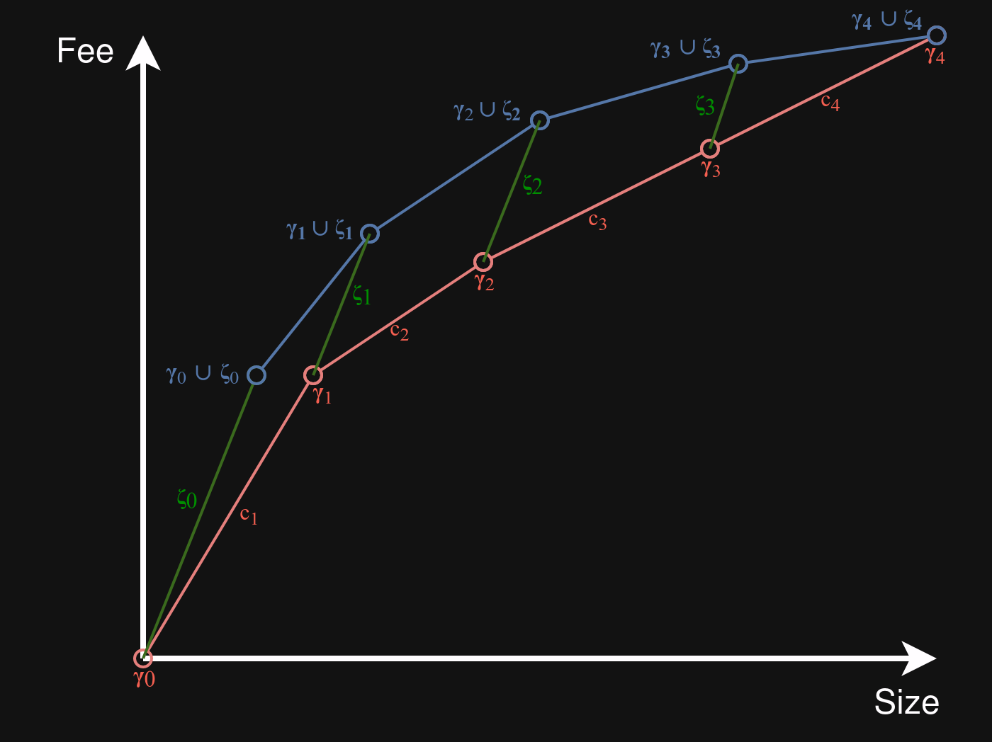
\operatorname{diag_L} is a concave function, which means it lies on or below each of its tangents. This implies that a point lies on or above the function iff it lies on or above at least one of its tangents. For every point on \operatorname{ndiag} we will identify a tangent of \operatorname{diag_L} that it lies on or above. As that function is made up of straight segments, its tangents are exactly these segments, extended to infinity in both directions.

• The points \{\forall \alpha \in [0, 1]: \alpha P(\zeta_0)\} lie on the first segment of \operatorname{ndiag}. We show they lie on or above the (extension of the) c_1 segment of \operatorname{diag}(L).
  • For \alpha=0, the functions coincide at (0, 0).
  • For \alpha > 0, the slope from (0,0) to P(\gamma_1) is \operatorname{feerate}(c_1) = f. The slope of the line from (0,0) to \alpha P(\zeta_0) is \operatorname{feerate}(\zeta_0) \geq f , which is at least as high.
• For i=0 \ldots n-1, the points \{\forall \alpha \in [0, 1]: (1-\alpha)P(\gamma_i \cup \zeta_i) + \alpha P(\gamma_{i+1} \cup \zeta_{i+1})\} lie on \operatorname{ndiag}. We show they lie on or above the (extension of the) c_{i+1} segment of \operatorname{diag}(L).
  • The slope of the c_{i+1} segment, from P(\gamma_i) to P(\gamma_{i+1}), is \operatorname{feerate}(c_{i+1}) \leq f.
  • For \alpha = 0, the slope of the line from P(\gamma_i) to (1-\alpha)P(\gamma_i \cup \zeta_i) + \alpha P(\gamma_{i+1} \cup \zeta_{i+1}) is \operatorname{feerate}(\zeta_i) \geq f.
  • For \alpha = 1, the slope of the line from P(\gamma_i) to (1-\alpha)P(\gamma_i \cup \zeta_i) + \alpha P(\gamma_{i+1} \cup \zeta_{i+1}) is \operatorname{feerate}(\zeta_{i+1} \cup c_{i+1}). Since \operatorname{feerate}(\zeta_{i+1}) \geq \operatorname{feerate}(c_{i+1}), it follows that \operatorname{feerate}(\zeta_{i+1} \cup c_{i+1}) \geq \operatorname{feerate}(c_{i+1}).
    • The one exception is i = n-1, as \zeta_n is empty there, and thus has no \operatorname{feerate}; this is not a problem as the functions coincide in this point.
  • The points with 0 < \alpha < 1 linearly interpolate between \alpha=0 and \alpha=1. Since both endpoints lie on or above the segment, the points in between also lie on or above the same segment.

Thus, \operatorname{ndiag}, an underestimate for the feerate diagram of L', is always at least as high as \operatorname{diag_L}, the feerate diagram of L. We conclude that L' \gtrsim L.

Merging linearizations

Definition. Let \operatorname{merge}(G, L_1, L_2) be the function on graphs G with valid linearizations L_1 and L_2, defined as follows:

• If G (and thus L_1 and L_2) are empty, \operatorname{merge}(\{\}, (), ()) = ().
• Otherwise:
  • Let (c_1, \ldots) = \operatorname{chunks}(L_1).
  • Let (c_2, \ldots) = \operatorname{chunks}(L_2).
  • If \operatorname{feerate}(c_1) > \operatorname{feerate}(c_2), swap L_1 with L_2 (and c_1 with c_2).
  • Let L_3 = L_1[c_2], the first chunk of L_2, using the order these transactions have in L_1.
  • Let (c_3, \ldots) = \operatorname{chunks}(L_3).
  • Let L_4 = L_3[c_3] = L_1[c_3], the linearization of the first chunk of L_3.
  • \operatorname{merge}(G, L_1, L_2) = L_4 + \operatorname{merge}(G \setminus c_3, L_1[G \setminus c_3], L_2[G \setminus c_3]).

Theorem. \operatorname{merge}(G, L_1, L_2) \gtrsim L_1 and \operatorname{merge}(G, L_1, L_2) \gtrsim L_2.

Proof.

The theorem is trivially true for empty G. For others, we use induction:

• First note that \operatorname{feerate}(c_3) \geq \operatorname{feerate}(c_1):
  • After the optional swapping step it must be the case that \operatorname{feerate}(c_2) \geq \operatorname{feerate}(c_1).
  • Further, \operatorname{feerate}(c_3) \geq \operatorname{feerate}(c_2), because L_3 contains the same transactions as c_2. If the \operatorname{chunks} operation on L_3 finds nothing better, it will pick the entirety of L_3 as c_3, which has the same feerate as c_2.
• Now define the following:
  • Let L_1' = L_4 + L_1[G \setminus c_3]. By the gathering theorem, L_1' \gtrsim L_1, as it is bringing a topologically valid sublinearization (L_4 = L_1[c_3]) to the front, and it has just a single chunk (c_3), whose feerate is \geq \operatorname{feerate}(c_1), the highest feerate in L_1.
  • Let L_2' = L_4 + L_2[G \setminus c_3]. By the chunk reordering them, L_2' \gtrsim L_2, as L_2' equals L_2 apart from its first chunk (c_3 \subset c_2).
• By the induction hypothesis, \operatorname{merge}(G \setminus c_3, L_1[G \setminus c_3], L_2[G \setminus c_3]) \gtrsim L_1[G \setminus c_3], and thus by the stripping theorem, L_4 + \operatorname{merge}(G \setminus c_3, L_1[G \setminus c_3], L_2[G \setminus c_3]) \gtrsim L_4 + L_1[G \setminus c_3] = L_1'. The same reasoning applies to L_2'.
• Put together, \operatorname{merge}(G, L_1, L_2) \gtrsim L_1' \gtrsim L_1 and \operatorname{merge}(G, L_1, L_2) \gtrsim L_2' \gtrsim L_2.

Variations. A number of variations on this algorithm are possible which do not break the proof above:

• Whenever a non-empty prefix P is shared by L_1 and L_2, it can be skipped (this follows directly from the stripping theorem), so if L_1 = P + A and L_2 = P + B, then one can define \operatorname{merge}(G, L_1, L_2) = P + \operatorname{merge}(G \setminus P, A, B).
• Instead of only considering the first chunk of L_2 in the order of L_1, it’s possible to also consider the first chunk of L_1 in the order of L_2, and then pick the first chunk of the one of those two which has the higher feerate.

Optimal linearizations

Definition. An optimal linearization/chunking for a graph is one which sorts higher or equal than every other linearization/chunking for the same graph. Note that this implies that optimal linearizations/chunkings are comparable with every other linearization/chunking. An optimal linearization/chunking is a greatest element of the set of all linearizations/chunkings of a graph.

Theorem. The set of linearizations/chunkings of a graph, with the preorder relation defined above, forms an (upward) directed set.

Proof. From the properties of the \operatorname{merge} algorithm it follows that for any two linearizations L_1 and L_2 there exists a L_3 = \operatorname{merge}(G, L_1, L_2) such that L_3 \gtrsim L_1 and L_3 \gtrsim L_2.

Theorem. Every graph has at least one optimal linearization/chunking.

Proof. In a directed set, every maximal element is a greatest element. Every finite preordered set has at least one maximal element. In a directed set, that element is a greatest element too.

Definition. For a given total ordering R_1 on the set of sets of transactions, and a total ordering R_2 on the set of sequences of transactions, define the function \operatorname{opt}_{R_1,R_2}(G), for a given graph G as follows:

• If G is empty, return the empty sequence: \operatorname{opt}_{R_1,R_2}(G) = ().
• Otherwise:
  • Let S be the highest-feerate subset of G. If there are multiple, pick the first one according to R_1.
  • Let L_S be the first valid linearization of S according to R_2.
  • \operatorname{opt}_{R_1,R_2}(G) = L_S + \operatorname{opt}_{R_1,R_2}(G \setminus S).

Theorem. \operatorname{opt}_{R_1,R_2}(G) is an optimal linearization of G.

Proof. Assume L = \operatorname{opt}_{R_1,R_2}(G) is not an optimal linearization of G. We already know an actual optimal linearization L_{opt} must exist though, so L_{opt} > L.

There must be a first chunk in the chunking of L where the fee-size diagram differs with L_{opt}. Let p be the set of all transactions in L in chunks before that point. Let L_{opt}' = L[p] + L_{opt}[G \setminus p], i.e. the linearization obtained by moving the diagram-equal L chunks to the front in L_{opt}. By repeatedly applying the gathering and stripping theorem, L_{opt}' \gtrsim L_{opt}. Because L_{opt} is optimal this implies L_{opt}' \sim L_{opt} > L. L_{opt}' and L both start with the same chunks, so by removing them we get L_{opt}[G \setminus p] > L[G \setminus p]. L[G \setminus p] = \operatorname{opt}_{R_1,R_2}(G \setminus p) however, and it starts by picking the highest-feerate subset of (G \setminus p), and yet L_{opt}[G \setminus p] starts with a better chunk. This is a contradiction.

For how to compute \operatorname{opt}(G) efficiently, see How to linearize your cluster.

Connected chunks

Definition. A connected chunking is a chunking for which each chunk is connected ignoring direction (i.e., given any transaction in a chunk, every other transaction in the same chunk can be reached when ignoring direction of the edges).

Theorem. In an optimal linearization/chunking, the corresponding chunks have connected components whose feerate is all the same. This is trivially true if the chunks are all connected.

Proof If not, the chunks could be split in two, which would improve the diagram.

Theorem. Every graph has at least one optimal linearization/chunking whose chunks are connected.

[murch]

@sipa

Definition. A chunking C = (c_1, c_2, \ldots, c_n)C=(c1,c2,…,cn)C = (c_1, c_2, \ldots, c_n) for a given graph G is a list of sets of transactions (called chunks) of G such that:

• The chunks c_icic_i form a partition of G (no overlap, and their union contains all elements).
• Every prefix of chunks is topological (\cup_{i=1}^{k} c_i∪ki=1ci\cup_{i=1}^{k} c_i for k=1 \ldots nk=1…nk=1 \ldots n are topological subsets of GGG). Thus, a transaction’s parent can appear in the same chunk as the transaction itself or in an earlier chunk, but not in a later chunk.
• The feerates of the sets are monotonically decreasing. Thus, the consecutive prefices of chunks form the highest, second-highest, … feerate topological prefices.

I assume you are defining it on a graph so that you can have a chunking across multiple clusters, but it seems to me that this definition would only require that the topology is valid at the chunk borders and would not require the transactions to be topological within the chunks. I think it would be correct if you said “every prefix of the chunking is topological” instead of “every prefix of chunks is topological”.

@sipa

Theorem. The corresponding chunking is a valid chunking, and is unique. The same chunking is obtained regardless of what order of merge operations is used. Thus, we can talk about the corresponding chunking \operatorname{chunks}(L)chunks(L)\operatorname{chunks}(L) of a linearization LLL. [no proof yet]

@sipa

For other values it linearly interpolates between those points.

Would it perhaps be sufficient that a feerate diagram has exactly one “convex hull” for a geometric proof? E.g. if we draw all transactions separately in the feerate diagram instead of their chunks, could we use the approach you use in the gathering theorem to show that all possible subgroupings will always be below the convex hull?

@sipa

Theorem. The chunk reordering theorem: reordering a linearization with changes restricted to a single chunk results leaves it at least as good.

Should this perhaps be restricted to topologically valid reorderings?

@sipa

Let e_j = c_j \cap Sej=cj∩Se_j = c_j \cap S for j=1 \ldots nj=1…nj=1 \ldots n, the SSS transactions in chunk iii of LLL. Note that this is distinct from d_jdjd_j because e_jeje_j follows the chunk boundaries of LLL, while d_jdjd_j follows the boundaries of L[S]L[S]L[S].

This should be “in chunk j of L”.

@sipa

Let \zeta_j = \cup_{i=j+1}^{n} e_iζj=∪ni=j+1ei\zeta_j = \cup_{i=j+1}^{n} e_i for j = 1 \ldots nj=1…nj = 1 \ldots n, the SSS transactions after the first jjj chunks of LLL.

Maybe “all remaining transactions of S after the first j chunks of L” would be clearer.

@sipa

Let SSS be the highest-feerate subset of GGG. If there are multiple, choose an arbitrary but consistent to order them.

“choose an arbitrary but consistent way/approach/method/criteria/something to order them”?

@sipa

Theorem. In an optimal linearization/chunking, the corresponding chunks have connected components whose feerate is all the same. This is trivially true if the chunks are all connected. Proof If not, the chunks could be split in two, which would improve the diagram.

Linebreak missing before the Proof.

I find that phrasing a bit confusing. What do you mean with “have connected components whose feerate is all the same”? I assume you are referring to the optimal linearization consisting only of chunks that cannot be split further by reordering, i.e. that any valid reordering would not lead to a different chunking, but the “have connected components whose feerate is all the same” makes me think that you are postulating that there are two chunks with the same feerate.

[sipa]

@murch

I assume you are defining it on a graph so that you can have a chunking across multiple clusters

Right. I’ve added a paragraph to elaborate on why that is.

@murch

it seems to me that this definition would only require that the topology is valid at the chunk borders and would not require the transactions to be topological within the chunks.

Chunks, as defined here, are sets; they don’t have an internal ordering. I’ve gone back and forth in my thinking whether sets or sequences are better. The advantage of sets is that at the chunking level, you don’t need to care about distinct intra-chunk linearization orderings. The disadvantage is that converting back from chunkings to linearizations isn’t as natural.

@murch

Would it perhaps be sufficient that a feerate diagram has exactly one “convex hull” for a geometric proof? E.g. if we draw all transactions separately in the feerate diagram instead of their chunks, could we use the approach you use in the gathering theorem to show that all possible subgroupings will always be below the convex hull?

Let me think a bit more about that.

@murch

Should this perhaps be restricted to topologically valid reorderings?

Done.

@murch

This should be “in chunk j of L”.

Fixed.

@murch

Maybe “all remaining transactions of S after the first j chunks of L” would be clearer.

Agreed, done.

@murch

“choose an arbitrary but consistent way/approach/method/criteria/something to order them”?

I’ve formalized this a bit more, selecting the ordering before the function definition.

@murch

What do you mean with “have connected components whose feerate is all the same”? I assume you are referring to the optimal linearization consisting only of chunks that cannot be split further by reordering, i.e. that any valid reordering would not lead to a different chunking, but the “have connected components whose feerate is all the same” makes me think that you are postulating that there are two chunks with the same feerate.

Consider the following cluster:

graph BT
   T0["B: 7"] --> T1;
   T1["A: 1"];
   T2["D: 5"] --> T3;
   T3["C: 3"];
   T4["E: 1"] --> T0;
   T4 --> T2;

• The linearization [ACDBE] has chunking [ACDB,E]
• The linearization [ABCDE] has chunking [AB,CD,E]

As defined so far, both linearizations are equivalent (because their diagram coincides), and optimal. Yet still, chunk ACDB contains two disconnected components. The point of this theorem is showing that in an optimal linearization, chunks are still not necessarily connected, but this is only possible if the connected components all have the same feerate (4 in this example).

What I want to get to here, but haven’t really fleshed out, is a stronger notion of optimality than defined so far, which also requires all chunks to be connected - and that every graph has such a very-optimal linearization too.

Actually, now that you bring it up, I realize that’s not as strong as we’d want yet. Even with requiring connected chunks, it’s still possible that optimal chunkings contain chunks with equal-feerate subsets, so I guess very-optimality should instead be “optimal diagram, and chunks cannot contain topologically-valid strict subsets with equal feerate as the chunk itself” or so?

[ajtowns]

@sipa

What I want to get to here, but haven’t really fleshed out, is a stronger notion of optimality

Isn’t this just about preferring (a) multiple smaller chunks to a single larger chunk, and (b) smaller chunks to be linearised before larger chunks, given the chunks have equal fee rates?

Is it possible to have two chunkings “A,B,C” and “D,E,F” where all have the same feerate, A is smaller than D, and DE is smaller than AB, and there is no alternative chunking “G,H,I” where G is smaller or equal to A and GH is smaller or equal to DE?

[sipa]

@ajtowns

Isn’t this just about preferring (a) multiple smaller chunks to a single larger chunk, and (b) smaller chunks to be linearised before larger chunks, given the chunks have equal fee rates?

I believe that is too strong - while we do want to consider breaking up chunks into multiple equal-feerate ones an improvement, I don’t think there is an objective reason to want the smallest ones first. (in my implementation, I do prefer smaller size when comparing equal-feerate transaction sets, but that’s an arbitrary choice that happens to prevent merging of such equal-feerate chunks).

One possibility, which I think is sufficient, is in the \gtrsim (& co) definitions is to use the total number of chunks as a tie-breaker when the fee-size diagram coincides exactly (more chunks = better). This has the advantage that “optimal linearization” automatically implies chunks which have no non-trivial subsets of the same feerate, and it doesn’t introduce a new source of incomparability. The disadvantage is that (as stated) it breaks the gathering theorem, and I suspect fixing that would complicate matters somewhat. That may also have implications for the prefix-merging algorithm’s proof (I believe the algorithm itself actually keeps its properties under this stronger ordering definition).

An alternative is leaving the preorder on linearizations alone, and instead only incorporate into the “optimal linearization” definition that chunks cannot have non-trivial subsets of higher or equal feerate. Alternatively, it could be a notion of “perfect linearization” which is stronger than optimal (and leave optimal to only be about the feerate diagram). This may be nicer in terms of presentation as the properties can be introduced and proven incrementally.

[ajtowns]

@sipa

I don’t think there is an objective reason to want the smallest ones first.

Oh, actually, I think you want the smallest ones last, if anything? (Or is my guess for getting mildly better performance out of greedy knapsack selection off the mark?)

Is this about optimising for the last few transactions in a block, or choosing a canonical ordering so there’s less uncertainty/ambiguity, or something else?

You can’t get a strictly unique “perfect” linearisation, since if you have txs A, B, C, C spending A and B, and A,B having equal fee and size, but lower feerate than C, then [ABC] and [BAC] are equally good linearisations. You could break the tie by resorting to your arbitrary order R_2, of course, but that’s still picking a winner arbitrarily…

Your definition of opt seems weird? Shouldn’t that just be \operatorname{opt}(G) = L_G + \operatorname{opt}(G \setminus S_G) where S_G is the highest-feerate subset of G and L_G is the first valid linearisation of S_G?

I would have proven the uniqueness claim non-constructively: set f(L) = |\{L_2 | L \ge L2\}|. Pick a linearisation L_x where f(L_x) \ge f(L) for all L. If this value equals the count of all linearisations, then L_x \ge L for all L, so L_x is an optimal linearisation. If it’s not the case, then there is some L_y where L_x \not\ge L_y, so calculate L_z = \operatorname{merge}(L_x, L_y) which gives us L_z \ge L_x but also L_z \ge L_y. But for any L where L_x \ge L, L_z \ge L by transitivity, so f(L_z) \gt f(L_x) which contradicts our choice of L_x.

[sipa]

@ajtowns

Oh, actually, I think you want the smallest ones last, if anything? (Or is my guess for getting mildly better performance out of greedy knapsack selection off the mark?)

Is this about optimising for the last few transactions in a block, or choosing a canonical ordering so there’s less uncertainty/ambiguity, or something else?

It’s about optimizing for the last few transactions in a block; the more chunks clusters are broken up in, the more puzzle pieces there are to use. I don’t think you can - without whole-mempool context - say whether the beginning or the end of a cluster is better to have small pieces, as you don’t know ahead of time where they’ll end up in a block. And I think the splitting itself is more important than the ordering.

@ajtowns

You can’t get a strictly unique “perfect” linearisation, since if you have txs A, B, C, C spending A and B, and A,B having equal fee and size, but lower feerate than C, then [ABC] and [BAC] are equally good linearisations. You could break the tie by resorting to your arbitrary order R_2R2R_2, of course, but that’s still picking a winner arbitrarily…

Yeah. I don’t think we need to pick a well-defined unique optimal.

@ajtowns

Your definition of optoptopt seems weird? Shouldn’t that just be \operatorname{opt}(G) = L_G + \operatorname{opt}(G \setminus S_G)opt(G)=LG+opt(G∖SG)\operatorname{opt}(G) = L_G + \operatorname{opt}(G \setminus S_G) where S_GSGS_G is the highest-feerate subset of GGG and L_GLGL_G is the first valid linearisation of S_GSGS_G?

I would have proven the uniqueness claim non-constructively: set f(L) = |{L_2 | L \ge L2}|f(L)=|{L2|L≥L2}|f(L) = |{L_2 | L \ge L2}|. Pick a linearisation L_xLxL_x where f(L_x) \ge f(L)f(Lx)≥f(L)f(L_x) \ge f(L) for all LLL. If this value equals the count of all linearisations, then L_x \ge LLx≥LL_x \ge L for all LLL, so L_xLxL_x is an optimal linearisation. If it’s not the case, then there is some L_yLyL_y where L_x \not\ge L_yLx≱LyL_x \not\ge L_y, so calculate L_z = \operatorname{merge}(L_x, L_y)Lz=merge(Lx,Ly)L_z = \operatorname{merge}(L_x, L_y) which gives us L_z \ge L_xLz≥LxL_z \ge L_x but also L_z \ge L_yLz≥LyL_z \ge L_y. But for any LLL where L_x \ge LLx≥LL_x \ge L, L_z \ge LLz≥LL_z \ge L by transitivity, so f(L_z) \gt f(L_x)f(Lz)>f(Lx)f(L_z) \gt f(L_x) which contradicts our choice of L_xLxL_x.

Yeah, that’s proving the existence of optimality through \operatorname{merge}. My thinking was to prove existence of optimality before introducing merging (because proving that “move best subset to the front, continue” is optimal seems more intuitive than through merging), but perhaps that’s an unnecessary detour.

An alternative way to prove that, I think, is as follows. Let M be the set of maximal elements of the set of valid linearizations for a given graph (maxima have no elements that compare strictly higher than them, but may have elements incomparable to them).

• If M = \{\}: impossible in a finite set (start with any element and keep picking a strictly larger element, eventually you end up in a cycle, which is impossible as it implies elements strictly larger than themselves).
• If M = \{m\}, then m is optimal. Again start with any element, and keep picking strictly larger elements. Each of these chains must end with m as it’s the only element with no larger ones. Thus, m > everything else.
• Otherwise M consists of two or more elements: merge them, and end up with something better than both. This is in contradiction with them being maximal elements.

[sipa]

TIL about directed sets: sets with a preorder \geq and the additional property that for any pair of elements (a, b) an element c exists such that c \geq a and c \geq b.

In a directed set, every maximal element (m is maximal if no x > m exists) is a greatest element (m is greatest if for every x it holds that m \geq x).

Linearizations (and chunkings) of graphs/clusters are directed sets (with \gtrsim as the direction). The merge-intersection algorithm computes the c mentioned above given a and b. The “move highest feerate subset to front, continue with remainder” algorithm by construction computes a maximal element, which is thus a greatest element. “Optimal linearization” is the name we have for greatest element.

[sipa]

I’ve incorporated this “directed set” idea. Existence of an optimal linearization now follows from the merging algorithm, and with that knowledge, a simpler proof is possible that \operatorname{opt}(G) is optimal.

[Crypt-iQ]

@sipa

By repeatedly applying the gathering and stripping theorem, L_{opt}' \gtrsim L_{opt}.

I’m a bit confused here; could you elaborate on how the gathering and stripping theorems are used here? Since the gathering theorem applies when a sublinearization is moved to the front, it alone doesn’t prove that L_{opt}' \gtrsim L_{opt} since L[p] is the ordering from L rather than from L_{opt}. I’m not sure where the prefix stripping theorem comes in, so I must be missing something.

[sipa]

You’re right, I’m skipping over a few steps here.

What is happening is that we’re starting from L_{opt}, and moving the prefix of L that feerate-diagram-coincides with it to the front of L_{opt} so that we can skip over that, and just compare the part where the diagram actually differs. If it were any more obvious than it is, it would suffice to say “without loss of generality, assume L and L_{opt} have a distinct first chunk feerate”. This part of the argument is just to show that it indeed is without loss of generality, because if there is a coinciding prefix, then applying the theorem to just the transactions not in that prefix still leads to a contradiction.

This prefix p may consists of multiple chunks of L. If it consisted of 0 chunks, there is nothing to do, as L'_{opt} = L_{opt} in that case. If p consists of a single L-chunk, then just applying the gathering theorem gives our desired result (because in that case p has a feerate at least as much (and in fact, exactly equal to) the first chunk of L_{opt}).

The difficulty is only when p consists of multiple chunks. But in this case, repeatedly applying the gathering theorem (to move one L-chunk worth of p subset to the front of L_{opt}) and the stripping theorem (to skip over the just moved part) gets the result. I’m happy to write it out more formally, but this informal description is perhaps more enlightening?

[Crypt-iQ]

@sipa

If p consists of a single L-chunk, then just applying the gathering theorem gives our desired result (because in that case p has a feerate at least as much (and in fact, exactly equal to) the first chunk of L_{opt}).

This is the part I’m having trouble with. Can the gathering theorem be used here even though L_{opt}' is moving a sublinearization of L to the front of L_{opt} rather than moving a sublinearization of L_{opt} to the front of L_{opt}?

[sipa]

Oh, you need to use the chunk reordering theorem too, I forgot that was a separate thing in my writeup.

So you move (a chunk of) p to the front of L_{opt}, and then reorder it according the order those transaction have in L (which is allowed as they form a chunk).