How to linearize your cluster

[sipa]

@stefanwouldgo

But this way or through normal propagation I will learn of the newly attached attacker transaction eventually. When I do, I do the calculation again and resubmit with a better linearization.

No, not necessarily. If the attacker makes many different versions of the attached transaction, that all conflict with each other, and races them all to the network, then every network participant will eventually learn one of them, but not all, “partitioning” the network into groups of nodes which have the same attacker transaction. And relay of other, honest, transactions across these partition boundaries will be harder if you require the sender to provide good linearization information, because it will be a requirement of linearization on a cluster the sender does not (exactly) have.

---

In other news, I have a working GGT implementation with max-height active node selection strategy (so, \mathcal{O}(n^2 \sqrt{m})): Commits · sipa/bitcoin · GitHub. It passes all tests, so I’m reasonably confident that it can actually optimally linearize from scratch. I’ll post more detailed benchmarks later, but my benchmarks for up to 64 transactions run in 5-15 µs, and up to 60 µs for up to 99 transactions. These numbers are comparable to the spanning-forest linearizarion algorithm I posted about in the other thread. It’s a bit slower (around 1.5x) than the numbers I had before adding the concurrent reverse execution, but maybe that’s not a terrible price for gaining a factor n in the worst case.

Counting how many iterations the algorithm actually performs, and extrapolating that to the worst case for 64 transactions predicts something in the “few ms” range, which is amazing performance for a background optimizer, but probably not acceptable for doing at relay time itself.

[stefanwouldgo]

@sipa

If the attacker makes many different versions of the attached transaction, that all conflict with each other, and races them all to the network, then every network participant will eventually learn one of them, but not all, “partitioning” the network into groups of nodes which have the same attacker transaction. And relay of other, honest, transactions across these partition boundaries will be harder if you require the sender to provide good linearization information, because it will be a requirement of linearization on a cluster the sender does not (exactly) have.

This is an interesting partitioning attack. First, the partitioning part is already possible now. But it doesn’t really hurt anyone as long as nobody needs to attach to the attacker txns. If anybody else needs to spend an attacker txn, that is a problem already now, because presumably your mempool won’t accept a txn that spends an unknown attacker txn (which conflicts with your version of the attacker txn), so propagation of the honest txn might become impossible. Package relay might fix this.

What would change if we required nontrivial chunkings/linearizations to be forwarded? The attacker might partition the network with not just single txns but entire clusters that differ (maybe just in id, or maybe in structure). OK, here is where it gets worse: if for some reason we need to attach to the entire cluster (not just the attacker part, it might be an earlier tx that we spend), we cannot propagate our attachment, because we can only optimize our linearization for the cluster version that we know. Again, package relay might fix this, because if the entire cluster is preferable to the competing attacker clusters (because we optimized it), it can replace all of them.

So I see this as an interesting attack that probably needs fixing through package relay. And you are right that requiring linearizations makes it worse in the sense that the attack now also works if we don’t need to attach directly to malleable attacker txns, which probably makes it much more problematic, say, for LN. However, it seems to me that in all cases, it can be fixed by relaying entire clusters.

Also, in the case that is different from today, where we don’t directly attach to attacker txns, it seems that simply merging the attacker linearization with ours should be optimal. If we can prove that, I don’t see why requiring linearizations makes things worse.

[stefanwouldgo]

I‘ve opened a new topic for the discussion on this attack here because I don’t want to clutter this topic further and because I believe it is of independent interest.

[Lagrang3]

I was implementing a proof of concept myself, just to get some understanding of GGT.

examples/maxfeerate-ggt.cpp

I will love to see through your code.

I think there might be a little optimization gain if we consider the fact that the graph is bipartite. Nodes have either a non-zero capacity arc with the source or the sink but not both. If we classify nodes this way, let’s say into set N1 (nodes connected to the source) and N2 (nodes connected to the sink) we also realize that we can ignore arcs that go from N1 to N1, and N2 to N2, why is that? because for any arc that connects nodes a and b (in N1 for instance) that arc either:

case 1, does NOT carry any flow in the final solution, so it can be ignored,

case 2, it DOES carry some flow, but that means that there exist some node c in N2 for which a and b have an arc with (by the dependency transitivity) so we might as well deviate that flow directly from a to c and not use arc a-b, this can be done since these arcs have infinite capacity.

Similarly with N2-N2 arcs.

I might be wrong though, but I think it is an interesting idea worth exploring.

[sipa]

Hmm, I think this works, but it has some caveats:

• Changes to \lambda during GGT recursion mean that transactions may move from the sink side of the partition to the source side; I believe this violates the condition that only sink-to-node and node-to-source capacities may change. If so, this means the factor n speedup on the worst case disappears.
• It means that the edges need to be expanded to their transitive closure (if A depends on B, and B depends on C, we need an edge from A to C as well). With complexities like \mathcal{O}(n^2 \sqrt{m}), this may be a slight worsening in practice, if we account for the fact that realistic clusters tend to have m = \mathcal{O}(n), but the full transitive closure may well have m = \mathcal{O}(n^2).

I do remember reading about specialized bipartite-graph min-cut algorithms, though…

---

@Lagrang3

I will love to see through your code.

I’ll do a writeup soon on the implementation and optimizations I came up with, but I’m still experimenting with a few ideas first (in particular, trying representing the edge data in n\times n matrix form, so bitsets can be used to match things more easily).

[stefanwouldgo]

This is a great observation. I’m not sure how useful it will be since it seems to imply that we’d have to replace each edge within N1 and N2 by an edge between those two sets. This paper points to a balancing algorithm for bipartite graphs that is typically faster than GGT, but worse on adversarially chosen instances, which is probably not what we want unless we can require chunkings to be broadcast.

[sipa]

I’m beginning to think that the spanning-forest linearization (SFL) algorithm is a better choice in general than the min-cut GGT algorithm, because while asymptotic complexity is worse (we don’t even have a proof that it terminates), it’s actually a lot more practical. It’s of course possible to combine the two, e.g., use GGT just for linearizing very hard clusters in a background thread, but it’ll practically be barely used I expect.

The reasons for choosing SFL over GGT and CSS (candidate set search, the old exponential algorithm which this thread was originally about) are:

• Anytime algorithm: it is possible to interrupt SFL at any point, and get a linearization out. The longer it runs, the better the result gets. This is also true for CSS, but less so for GGT as any min-cut that has not been computed completely may not result in an improvement (and the entire runtime may consist of just a single cut).
• Improving existing linearizations: it is possible to initialize SFL with an existing linearization as input, and any output it gives will be a linearization that’s better or equal. In some, but not all, practical cases it makes the algorithm also find the optimal faster when provided with a good input linearization already. This avoids the need to use the linearization merging algorithm to combine with existing linearization, or the LIMO algorithm to combine candidate finding with improvement of an existing linearization.
• Load balancing: both GGT and CSS subdivide the problem in different ways. When trying to turn them into anytime algorithms, there is a question of how to subdivide the computation budget over these subproblems. In contrast, SFL always just operates on a single state which it keeps improving, so no such budgetting decisions are necessary.
• Fairness: Related to the previous point, it is easy to make SFL spread its work over all transactions in the cluster in a more-or-less fair way, for example by trying going through the transactions in a round-robin fashion to find dependencies to improve. GGT works by subdividing the cluster in a divide-and-conquer manner, but choices need to be made about which part to attempt to subdivide next. CSS fundamentally works from highest-feerate to lowest-feerate chunks, so if time runs after only some part is done, the (transactions in) the first chunk will have had more effort on them. I think that’s concerning, because it risks an attacker attaching a very complex set of transactions to an honest CPFP or so, and have the algorithm spend all its time on the attacker’s transactions, running out before even considering the steps necessary to recognize the CPFP.
• Runtime: when benchmarking using replayed mempool data of previous years (credit to @sdaftuar), my SFL implementation seems somewhat (~2x) faster than the GGT one.
• Integer arithmetic: GGT needs to represent flows and feerates as approximate integers, which need to be scaled such that they are sufficiently precise. If F is the sum of the (absolute values of) fees in the graph and S the sum of the sizes in the graph, then GGT needs integers large enough to represent 4S^2F if exactly optimal solutions are desired. SFL and CSS only need integers large enough to represent 2SF and SF. Of course, perhaps we don’t care about exactness of solutions for huge clusters that pay enormous feerates, and in either case, this isn’t a very hard problem, just complicates the implementation somewhat.

The downsides of SFL compared to GGT are:

• Complexity bounds: there is no known bound for the runtime of SFL, and it may be infinite, while GGT is proven to be \mathcal{O}(n^3). I suspect that SFL is \mathcal{O}(n^5) or so in the worst case. However, even GGT’s cubic runtime is probably too much in the worst case to run at transaction relay time. Also note that we don’t really need optimal linearization. They’re nice, because they’re obviously the most incentive-compatible ones, but in practice, the bar is really a “good enough for what people actually use”, which is hard to define, and interacts in difficult ways with adversial models (see fairness above).

The downsides of SFL compared to CSS are:

• Mix with ancestor sort: CSS, when used through LIMO, can include arbitrary additional sources for finding good topological sets to move to the front. In the current implementation, optimal ancestor sets are used as additional inputs. There are no well-defined properties that this gives the linearization, but at least intuitively, this provides a “linearization always has at least ancestor-set like quality” property, regardless of how much time was spent in candidate finding. I don’t know how to do anything like this in SFL (nor in GGT). If we believe that this quality is important, despite not being well-defined, then switching to SFL in theory means we could lose it in clusters that cannot be linearized optimally in time. My thinking is that combined with the SFL fairness, and the fact that it is just so much faster overall, it is unlikely to be an issue. Further, if we really wanted ancestor-sort quality, it would be possible to compute, in addition to running SFL, an ancestor sort linearization from scratch, and then merge the two if SFL doesn’t find an optimal result. However, I suspect that the time this would take is better spent on performing more SFL iterations.
• Minimal chunks: CSS finds a linearization by actively searching for good chunks to move to the front, and in doing so, it can prefer smaller chunks over bigger ones. This guarantees that (if it completes) it will find the linearization with minimal possible chunks among all feerate-diagram-optimal linearizations. SFL (and GGT) on the other hand really just find groups of connected transactions with equal chunk feerate, and thus can’t guarantee to pull equal-feerate chunks apart.
• Complexity bounds: there is no known bound for the runtime of SFL, and it may be infinite, while CSS is trivially bounded by \mathcal{O}(n \cdot 2^n), although I believe it may be \mathcal{O}(n \cdot \sqrt{2^n}) instead. These bounds are obviously impractical.

All 3 above issues are open questions, and solutions/improvements could be found to them.

---

In table form:

Trait		CSS		SFL		GGT
Proven worst-case		\mathcal{O}(n \cdot 2^n)		\mathcal{O}(\infty)		\mathcal{O}(n^3)
Conjectured worst complexity		\mathcal{O}(n \cdot \sqrt{2^n})		\mathcal{O}(n^5)		\mathcal{O}(n^3)
Historical avg. runtime (µs) (n \leq 64)		80		10		22
Historical worst runtime (µs) (n \leq 64)		31500		26		33
Extrapolated worst runtime (µs) (n \leq 64)		700,000,000		1,000,000		10,000
Anytime algorithm		Needs budgeting		Natively		May lose progress
Improving existing		Through LIMO		Natively		Merging afterwards
Fairness		Hard		Easy		Hard
Integer sizes		SF (\times,<)		2SF (\times,<,-)		4S^2F (\times,/,<,+,-)
Ancestor sort mix		Yes		No		No
Minimal chunks		Natively		No		No

[murch]

Cool results regarding SFL. It sounds quite attractive that you can just stop anytime and are guaranteed to have been at least as good as what you started with. If you remember whether a cluster is linearized optimally, it would be easy to pick up non-optimally linearized cluster at a later time and improve them in the background.

@sipa

Improving existing linearizations: it is possible to initialize SFL with an existing linearization as input, and any output it gives will be a linearization that’s better or equal.

@sipa

Mix with ancestor sort: CSS, when used through LIMO, can include arbitrary additional sources for finding good topological sets to move to the front. In the current implementation, optimal ancestor sets are used as additional inputs. There are no well-defined properties that this gives the linearization, but at least intuitively, this provides a “linearization always has at least ancestor-set like quality” property, regardless of how much time was spent in candidate finding. I don’t know how to do anything like this in SFL (nor in GGT).

I’m confused, I thought that CSS basically starts from the Ancestor Set Sort result, or it is guaranteed to be as good as Ancestor Set Sort by merging. If you have to do an Ancestor Set Sort to achieve at least Ancestor Set Sort quality, wouldn’t it be fair to do Ancestor Set Sort first and let SFL start with the result of Ancestor Set Sort?

[sipa]

@murch

I’m confused, I thought that CSS basically starts from the Ancestor Set Sort result, or it is guaranteed to be as good as Ancestor Set Sort by merging. If you have to do an Ancestor Set Sort to achieve at least Ancestor Set Sort quality, wouldn’t it be fair to do Ancestor Set Sort first and let SFL start with the result of Ancestor Set Sort?

There are multiple ways of combining things, but that is not how it’s currently implemented. The important part is that in practice, we have a linearization for every cluster at all times, and want to exploit that knowledge. So the input linearization to LIMO/CSS is the earlier, existing, linearization for the cluster, not a pure ancestor sort based linearization. This input linearization can be great (if it was a hard cluster that was linearized before, and only a trivial change made to it), but it may also be terrible (say two clusters got merged, so we combine their linearizations naively, but the transactions interact a lot).

The ancestor sort mixing-in happens inside, which means that each candidate set search can be bootstrapped from it, and LIMO’d with it.

The LIMO/CSS as implemented now, is roughly:

• Linearize(cluster, input_lin):
  • While cluster is not empty:
    • Find anc, the best ancestor set in cluster
    • Find pre, the best prefix of input_lin in what remains of cluster.
    • Set best = higher feerate of anc and pre
    • Update best = CSS(cluster, best), starting with best as initial candidate.
    • Update best to be the highest-feerate prefix of the intersection between best and input_lin (this is the LIMO step, guaranteeing that the result will be as good as input_lin).
    • Output best, and remove it from cluster

This mixing/bootstrapping with ancestor sets in addition to existing prefixes doesn’t actually guarantee anything (in particular, it does not guarantee that the output is as good as pure ancestor set sort, though in practice it’ll usually beat it easily), but it’s a relatively fast way to have a good initial thing to start with, in particular when the input linearization is terrible.

And it’s this incremental mixing in of various sources of candidate sets (whether that’s ancestor sets or CSS or something else) that I don’t know how to map to SFL. It can start with an input linearization, but I think it’s more important to use the existing cluster linearization for that. However, unless we really think that this ancestor-set mixing has some specifically useful properties, I don’t think we care. The normal SFL steps seem to make the output linearization very quickly better, and in practice, optimal within 10s of microseconds.

[gmaxwell]

There are also other non-GGT algorithms in the literature with similar worst case complexity. Perhaps one of them may even be (a variation of) SFL.

The factor of 2 is interesting to me, since that’s also what GGT loses from having to run both forward and backward to save a factor of N in the worst case-- right? If so leaving that out would leave it competitive with SFL in average performance but still better than SFL’s conjectured worst case.

I confess that I’m happy to see you seemingly leaning towards SFL because GGT’s arithmetic struck me as particularly ugly.

Preferring linearizations with smaller chunks first among options with equivalent feerate diagrams sounds pretty attractive particularly absent any kind of just in time space constrained linearization. But how often does it even matter historically? My WAG is that it’s almost always the case in practice that the optimal diagram is unique unless transactions are the same sizes.

[sipa]

@gmaxwell

There are also other non-GGT algorithms in the literature with similar worst case complexity. Perhaps one of them may even be (a variation of) SFL.

SFL is ultimately a modified version of simplex for the LP formulation of the maximum ratio closure problem, though one with two important changes:

• Whenever dependencies are made active (i.e., become basic variables in simplex terms), pick the ones whose feerate difference is maximal. This is crucial apparently, because (as far as fuzzing can confirm) it is sufficient to never hit repeated states.
• Operate on all chunks at once, rather than just on finding the one first chunk. This is nice from a computation perspective (no separation into subproblems that the budget needs to be split over), but also from a fairness perspective (can distribute work over all transactions equally).

Simplex in general, without heuristics, can cycle forever. With heuristics, it can be exponential in the worst case. But our problem is very much not a general LP problem, and the max-feerate-difference heuristic is a fairly strong one, so I think it’s at least plausible this makes it polynomial.

@gmaxwell

The factor of 2 is interesting to me, since that’s also what GGT loses from having to run both forward and backward to save a factor of N in the worst case-- right? If so leaving that out would leave it competitive with SFL in average performance but still better than SFL’s conjectured worst case.

I think I saw a factor of 1.5 from running forward and backward, but this is perhaps a good thing to include in further benchmarks, to compare SFL with a version of GGT that just runs forward (which has \mathcal{O}(n^4) worst-case complexity, FWIW).

And of course, these are tiny constant factors. They may also be achievable by mundane implementation aspects, like picking a different data structure here or there. Or they may be the consequence of a dumb oversight in my unreviewed implementations.

@gmaxwell

I confess that I’m happy to see you seemingly leaning towards SFL because GGT’s arithmetic struck me as particularly ugly.

I think SFL is more elegant too, mostly because it really has a small amount of state: the set of active edges. The implementation does need a lot of precomputed values to be efficient, but those precomputed values can all be determined in \mathcal{O}(n^2) time from the set of active dependencies. On the other hand, GGT has a lot of state: the flows between the source/sink and each transactions, and the flows along every dependency, and a copy of all of that per instance of the min-cut problem. It just feels like there is redundancy in there that is not exploited (e.g., there can be many equivalent flows that represent the same cut).

@gmaxwell

Preferring linearizations with smaller chunks first among options with equivalent feerate diagrams sounds pretty attractive particularly absent any kind of just in time space constrained linearization.

All else being equal, we should of course prefer smaller chunks over bigger ones, as it reduces the binpacking loss at the end of a block (it can be compensated through other means too, but if it can be done through smaller chunks it’s just a win overall). But on the other hand, exactly equal feerate chunks are just a special case. If we seriously cared about the binpacking impact of larger chunks, we should arguably also prefer splitting up “chunks” into quasi-chunks that have almost the same feerate. Unfortunately, that does break some of the theory (e.g., now it is no longer the case that chunks are monotonically decreasing in feerate), but as long as we’re talking about small feerate differences, this may still well be worth it in practice.

@gmaxwell

But how often does it even matter historically? My WAG is that it’s almost always the case in practice that the optimal diagram is unique unless transactions are the same sizes.

I have certainly seen clusters with many exactly-equal transaction fees and sizes.

[sipa]

Benchmark results

All data is tested in 6 different linearization settings:

• CSS: the candidate-set search algorithm this thread was initially about, both from scratch and when given an optimal linearization as input already.
• SFL: the spanning-forest linearization algorithm, also from scratch and when given an optimal linearization as input already.
• GGT: the parametric min-cut breakpoints algorithm from the 1989 GGT paper, both its full bidirectional version, and a variant that only runs in the forward direction.

Simulated 2023 mempools

This uses clusters that were created by replaying a dump of 2023 P2P network activity into a cluster-mempool-patched version of Bitcoin Core (by @sdaftuar), and storing all clusters that appear in a file. This included 199076 clusters of size between 26 and 64 transactions, and over 24 million clusters between 2 and 25 transactions. Note that this is not necessarily representative for what a post-cluster-mempool world will look like, as it enforces a cluster size limit of 64, which may well influence network behavior after adoption.

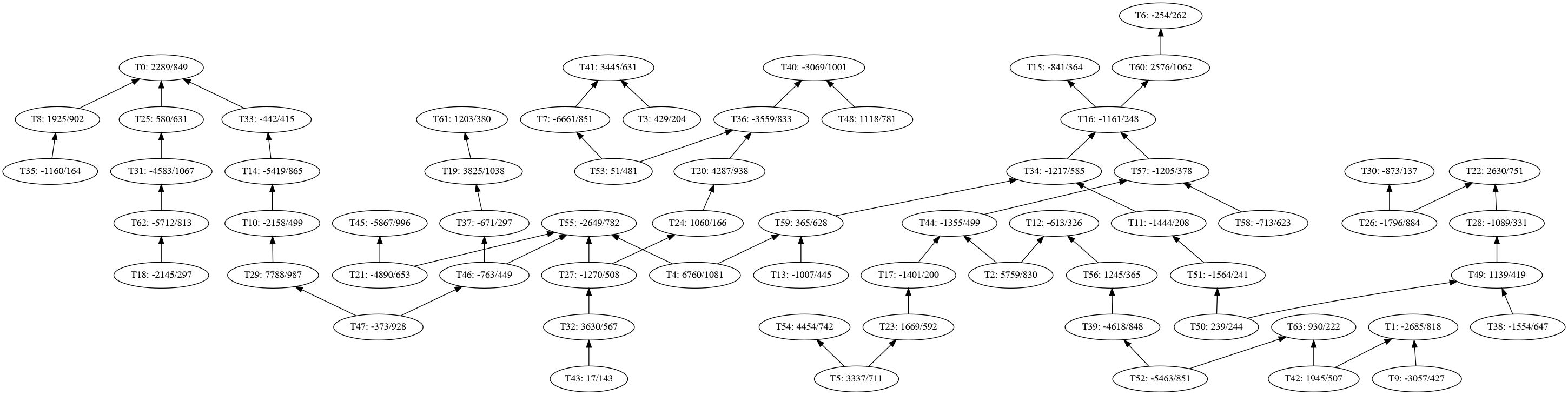
Here are two example 64-transaction clusters:

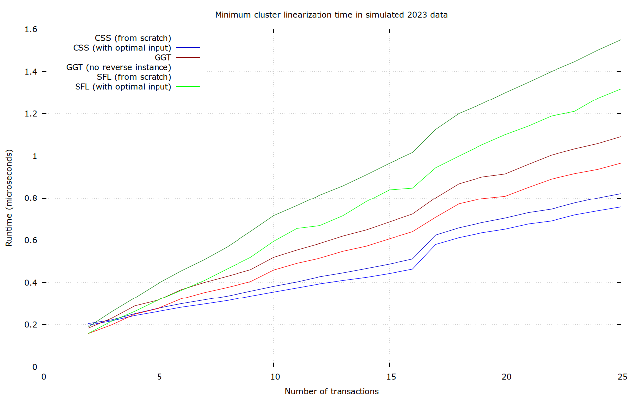
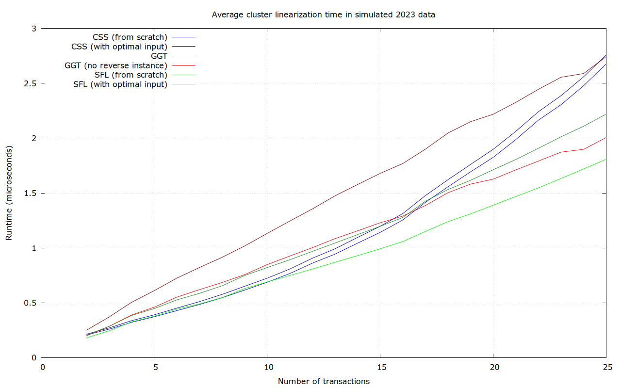
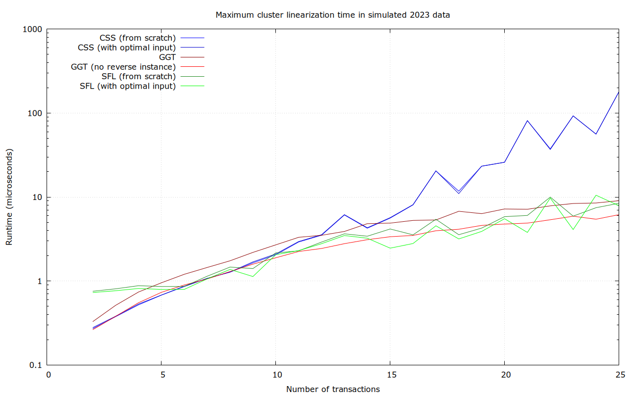
Numbers for 2-25 transaction clusters, based on benchmarks of 7.5% of the recorded clusters:

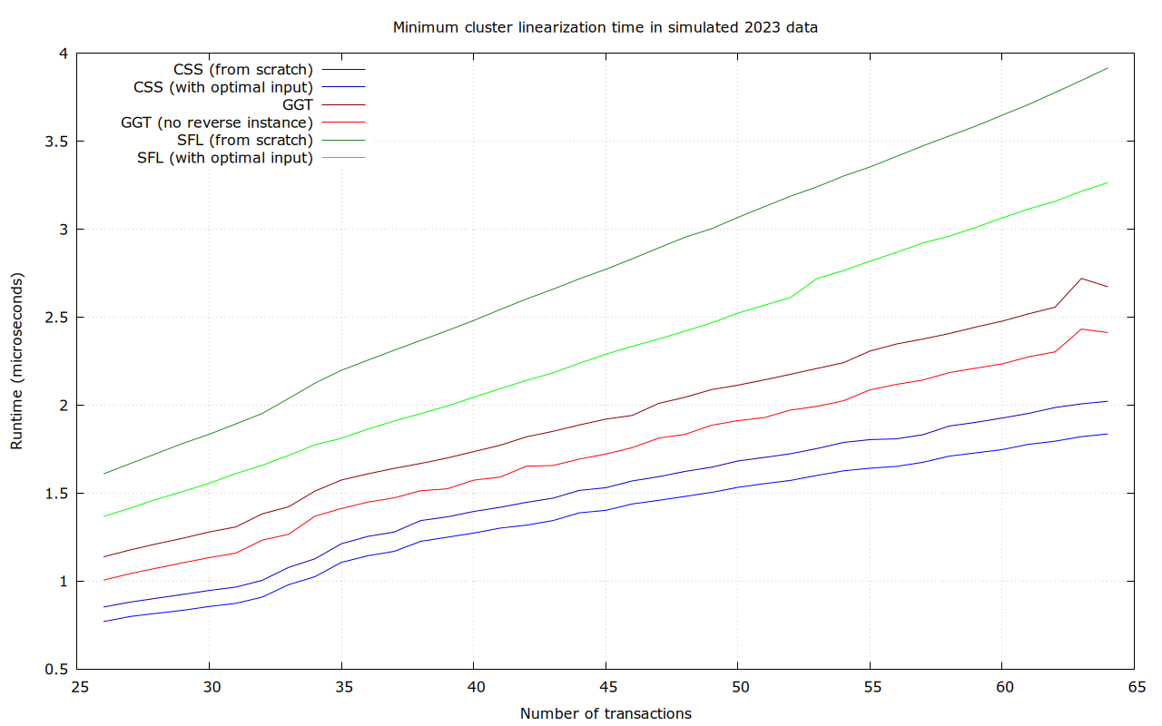
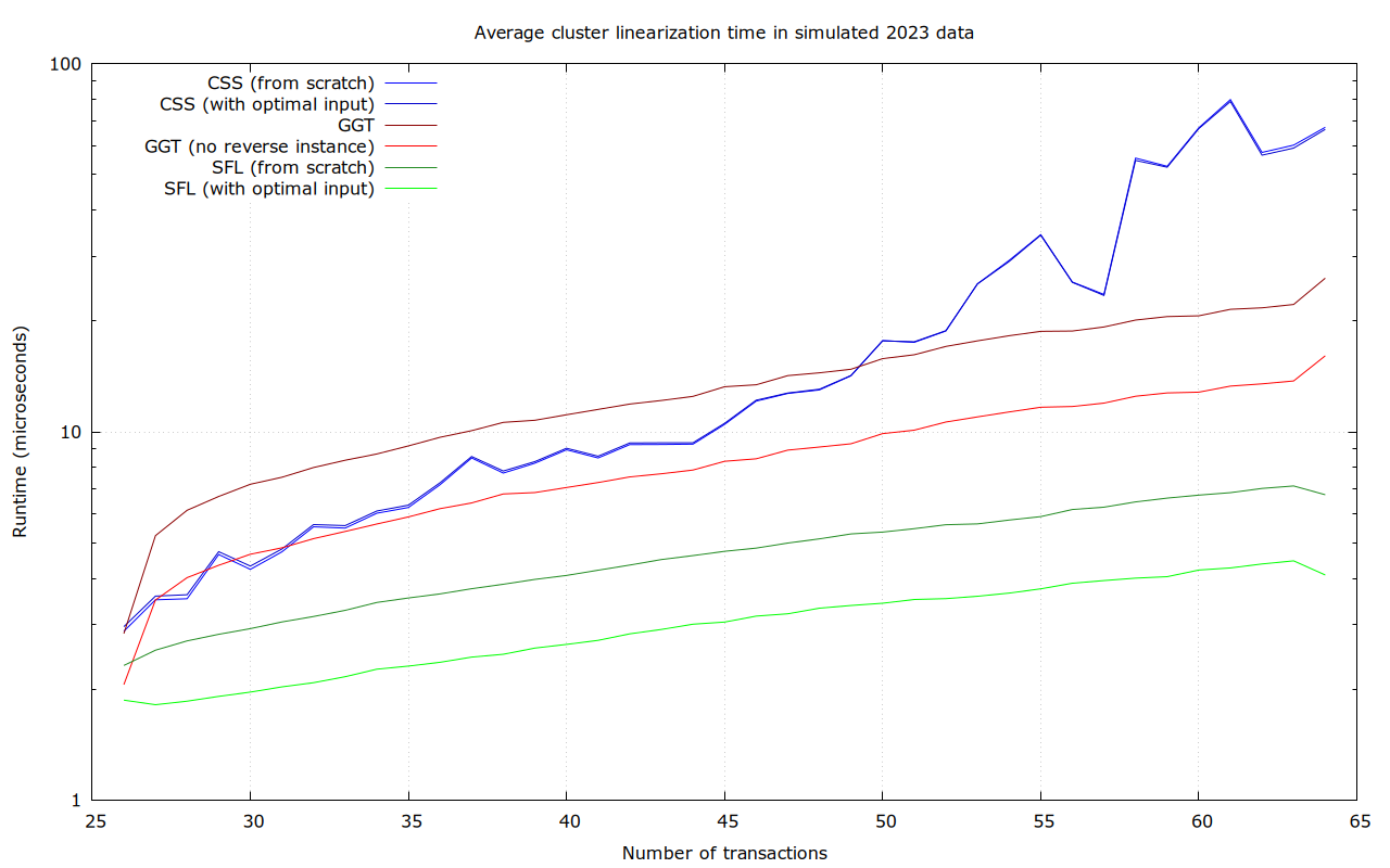
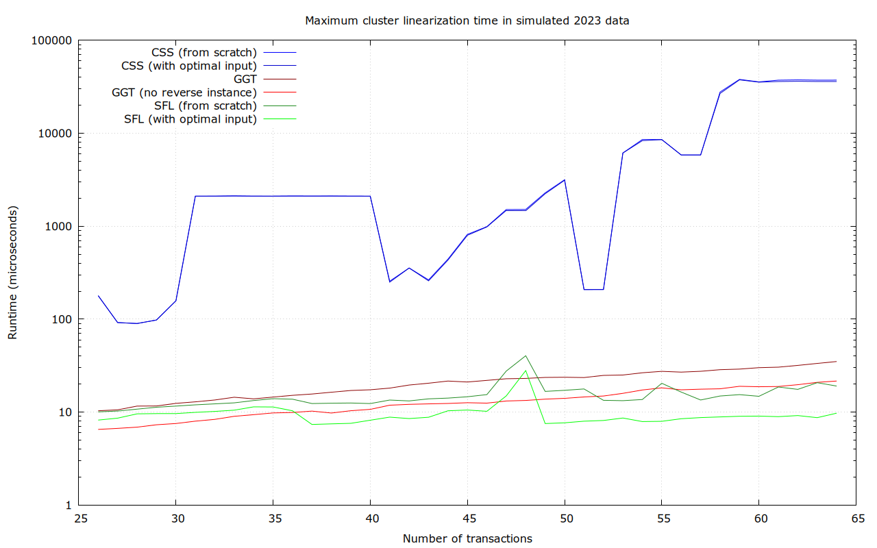
Numbers for 26-64 transaction clusters, benchmarking all of the clusters:

For sufficiently large clusters, and in average and maximum runtime, SFL is the clear winner in this data set. CSS has better lower bounds, but is terrible in the worst case (31.5 ms).

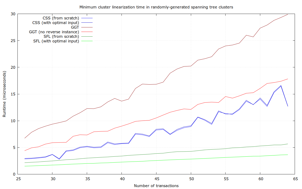
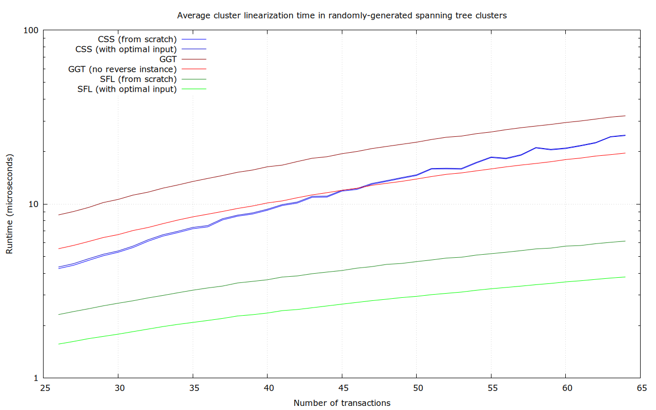
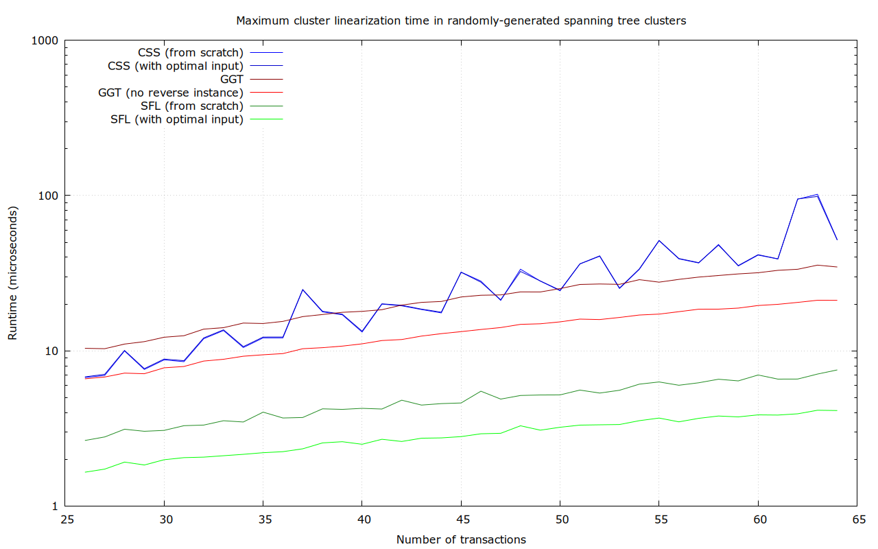
Randomly-generated spanning-tree clusters

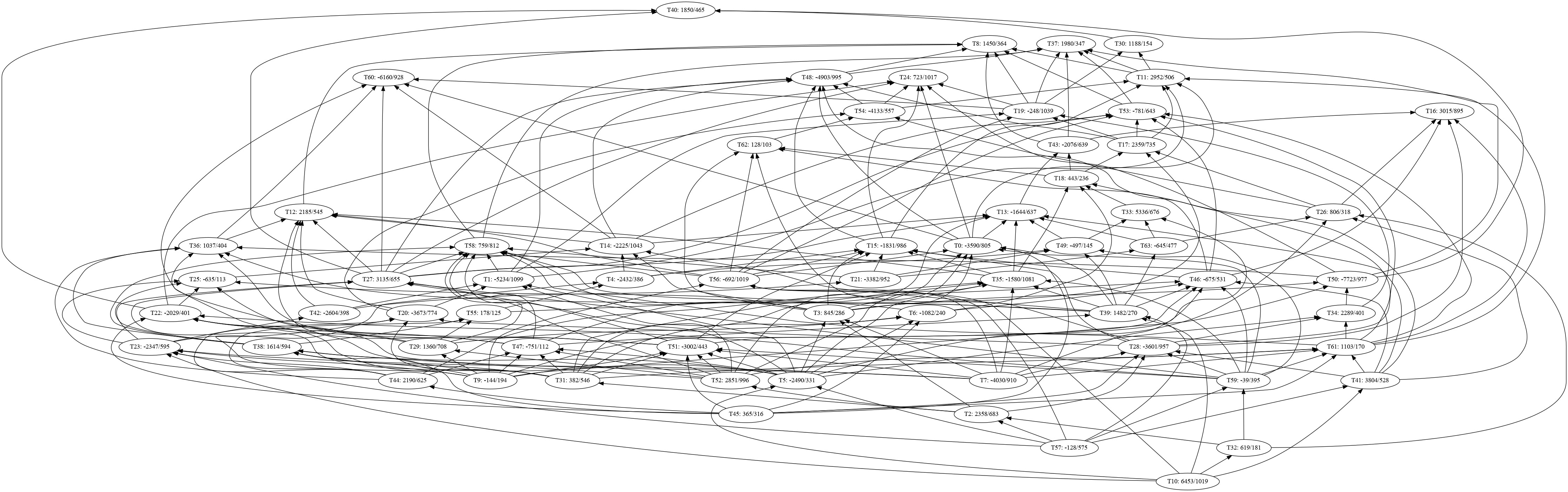
In this dataset, for each size between 26 and 64 transactions, 100 random spanning-tree clusters (i.e., a connected graph with exactly n-1 dependencies) were generated, like this 64-transaction one:

Again, SFL seems the clear winner.

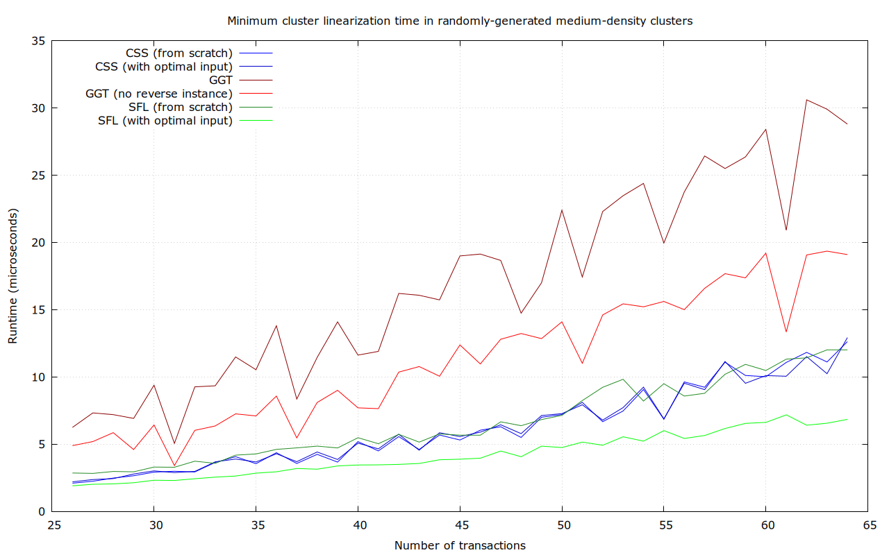
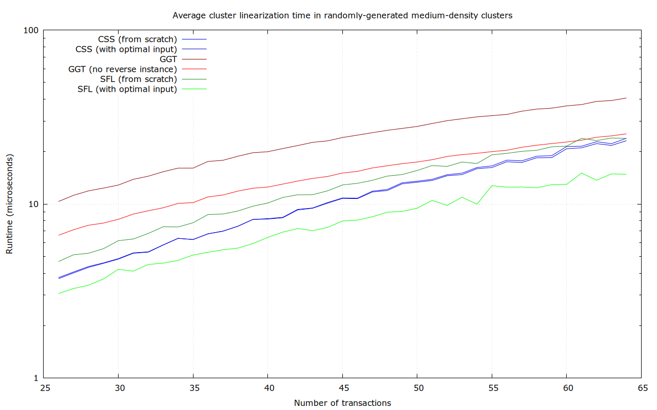
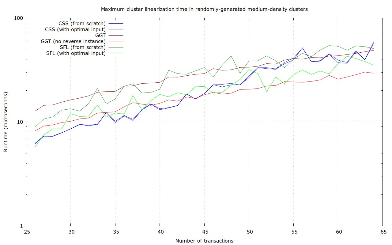
Randomly-generated medium-density clusters

In this dataset, for each size between 26 and 64 transactions, 100 random spanning-tree clusters (with roughly 3 dependencies per transaction) were generated, like this 64-transaction one. I promise this is not the plot of Primer (2004):

Notably, SFL performs worst in the worst case here, with up to 83.1 μs runtime, though even the fastest algorithm (unidirectional GGT) even takes up to 30.2 μs. This is probably due to it inherently scaling with the number of dependencies.

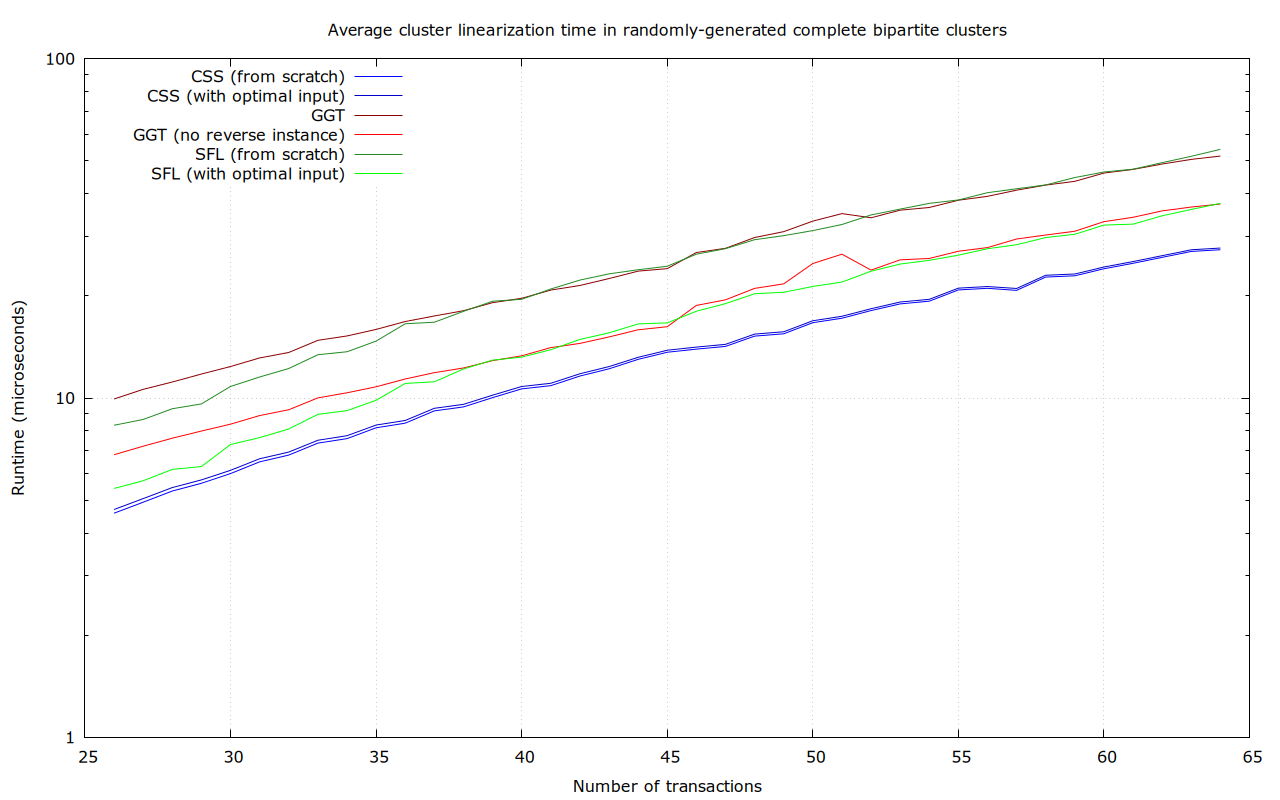
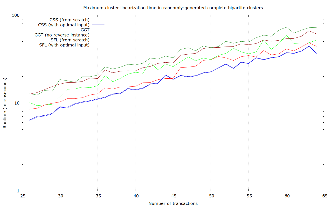
Randomly-generated complete bipartite clusters

In this dataset, for each size between 26 and 64 transactions, 100 random complete-connected bipartite clusters (with roughly n/4 dependencies per transaction) were generated, like this 64-transaction one:

With even more dependencies per transaction here, SFL’s weakness is even more visible (up to 114.8 μs), though it affects GGT too. Note that due to the large number of dependencies, these clusters are expensive too: if all the inputs and outputs are key-path P2TR, then the 64-transaction case needs ~103 kvB in transaction input & output data.

Methodology

All of these numbers are constructed by:

• Gather a list of N clusters (by replaying mempool data, or randomly generating them).
• For each of the N cluster, do the following 5 times:
  • Generate 100 RNG seeds for the linearization algorithm.
  • For each RNG seed:
    • Benchmark optimal linearization 13 times with the same RNG seed, on an AMD Ryzen 9 5950X system.
    • Remember the median of those 13 runs, to weed out variance due to task swapping and other effects).
  • Remember the average of those 100 medians, as we care mostly about how long the duration of linearization many clusters at once is, not an individual one. This removes some of the variance caused by individual RNG seeds.
• Output the minimum, average, and maximum of those 5N average-of-medians.

All the data and graphs can be found on Cluster linearization databench plotting code · GitHub.

[gmaxwell]

Time per ‘cost’ might be an interesting graph-- given that dependencies add transaction size. I had previously wondered if it might make sense for the limit to actually be in terms of dependencies rather than transactions in a cluster (e.g. set the limit to tx+dep < 512 or something).